Last Updated: 24 May 2024
Table of Contents
Abstract
Random forest and Bayesian Additive Regression Trees (BART) are algorithms considered as optimal supervised learning, non-parametric modeling techniques, each offering powerful tools for predictive analytics. I will explore each algorithm process and methodology for handling prediction and classification. Random forests generate numerous trees using tuning parameters that influence the number of trees and the complexity of each decision/split. BART, like Random forest, creates a number of trees, but applies a Markov-Chain Monte-Carlo process to determine an optimal set of trees to be summed (and not averaged like Random Forest). BART additionally incorporates Bayesian priors that govern the depth of each tree and the variety of node (leaf) values. Random forest mitigates overfitting by employing bootstrapping, generating unique datasets for each tree, and refining tree structures through Out-of-Bag (OOB) predictions. In contrast, BART utilizes regularization priors that penalize complex trees, ensuring that default priors favor non-null but small trees to prevent overfitting. We investigate how altering these tuning parameters (and priors) determine fit and prevent overfit on different predictive learning tasks. We apply both approaches to predicting knee angle from a suite of noisy sensors. For our scenarios, I find that BART demonstrates a slight superiority over random forest on 2 of our 3 examples, showcasing enhanced generalization to new observations, and emerges as a more compelling choice for predictive accuracy, despite its computational complexity. However, Random Forest is preferred in scenarios involving unique metrics (see knee sleeve example).
Introduction
Tree-Ensemble Models (including Random Forest and BART) rely on multiple decision trees to generate predictions. A classic decision tree contains several different branches (TRUE/FALSE decisions) and nodes (endpoints or values) that contribute to explaining some portion of a data problem, such that certain outcomes are expected when running through the tree. Because a tree can have many different combinations of branches/splits, using the tree for this purpose becomes a very viable and flexible method. However, using only one tree may fail in predicting on new data (overfitting). When multiple trees are used in a tree-ensemble model, their combining embodies that original flexibility of one tree AND prevents overfit. These two aspects is what makes Random Forests and BART very powerful tools.
Random Forest and BART are considered supervised forms of learning. They utilize nonparametric (flexible) approaches to modeling data without requiring the data to follow any particular form. Tree-based ensemble methods can be a reliable friend when your goal is to perform a machine learning task, and you lack the knowledge in (or motivation to research) the topic/data. However, these methods are not recommended for inference-related questions: using numerous trees restricts the interpretability of your data. But, the power from tree-ensemble models are in their ability to estimate predictions individually and combine them.
Random Forests and BART capitalize on the beauty of utilizing multiple decision tree models to increase predictive accuracy, but have notable differences on how they do so. While both tree-ensemble methods adjust their trees to reduce the amount of impurity, or error, within a fit, the fitting process for each contain many key differences. We will elaborate more on how these two methods generate and fit decision trees on data, how they can each be adjusted using tuning (hyper) parameters, how they relate in computation time, and also how they perform on some different predictive learning tasks.
Random Forest
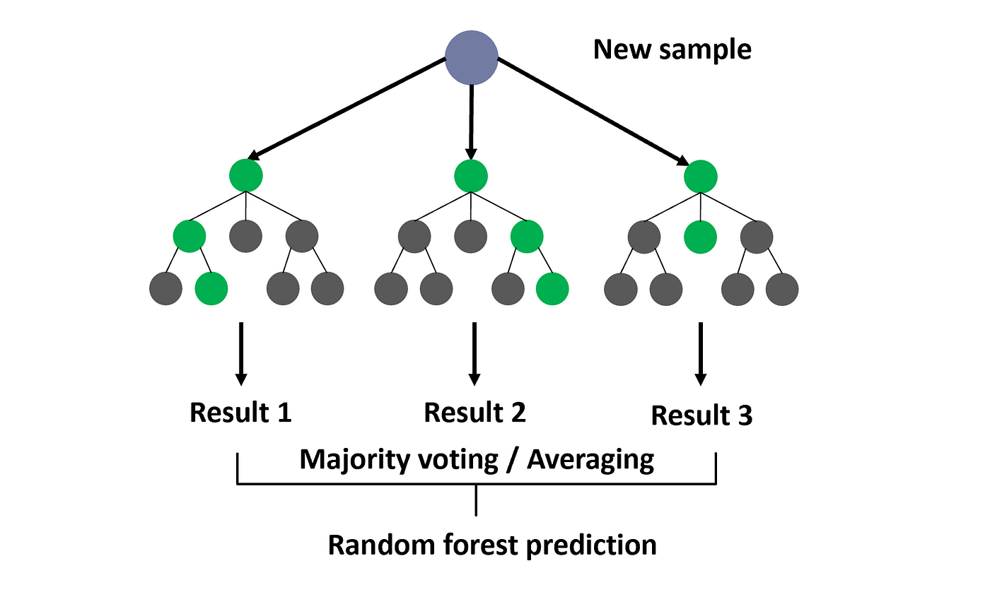
Random forests create multiple trees that are meant to cover the entire dataset. Dependent upon the task being classification or regression, each tree makes an independent decision about an observation, which then contribute to an aggregate value. This value is either a chosen class from a tree-majority vote, average probability of being within a certain class, or an average value from all trees (regression).
Random forests employ a technique called bootstrapping to generate an optimal set of trees. Bootstrapping takes random samples of the entire datset and creates each decision tree from that sample. The data not utilized for each tree is then used for calculating the out-of-bag predictions. The random forest model aims to create these trees such they still use the sampled data but minimize the out-of-bag error, as seen in the formula below. This metric prevents random forests from overfitting.

Random forests depend on the branch/leaf structure of each tree to assess how conservative/aggressive the fit is to the training data. A complex tree will feature more splits and more node values to represent possible values. When the number of splits increase, this forces the tree to represent more variations in the data, leading to an overfit. In addition, splits within trees are randomly considered from a subset of m of the p features within the data. The value of m does not change between each tree in the random forest model, but the variables within those m do. This is why the method is called “random forest”, as each tree randomly uses only a subset of the available features for splitting decisions.
The nature of how Random Forests makes splits depends on certain metrics involving “impurity node” values. These determine how well each split represents the bootstrap sample for a tree. Random Forests typically default to the Gini Index to measure how well it splits, which uniquely determines of all the possible variables to split, which one would have the lowest “impurity,” or the best data representation on each sides of the branch. Gini Index will pick the lowest impurity from the m variables selected for that tree.
Tuning Parameters
The tuning parameters in R that I mainly focus on are called ntrees, mtry, and nodesize.
ntreesdictate the number of trees in the model, where each tree contributes to the average value or class decision.mtrydetermines a random subset of the p features to fit for each tree. Default setsmtrytop/3for numerical targets orsqrt(p)for categorical targets.nodesizeis the minimum size for a terminal node to be created within a tree. Settingnodesizehigher will create smaller trees.
For more on the RandomForest() model in R, see the following documentation.
Computation Time
Compputation time for random forest models vary significantly depending on the complexity of the target, the dimensions of the training data, and the types of hyperparameters utilized for fitting. Even though random forests prove to be very powerful models, they surprisingly take very little time to generate.
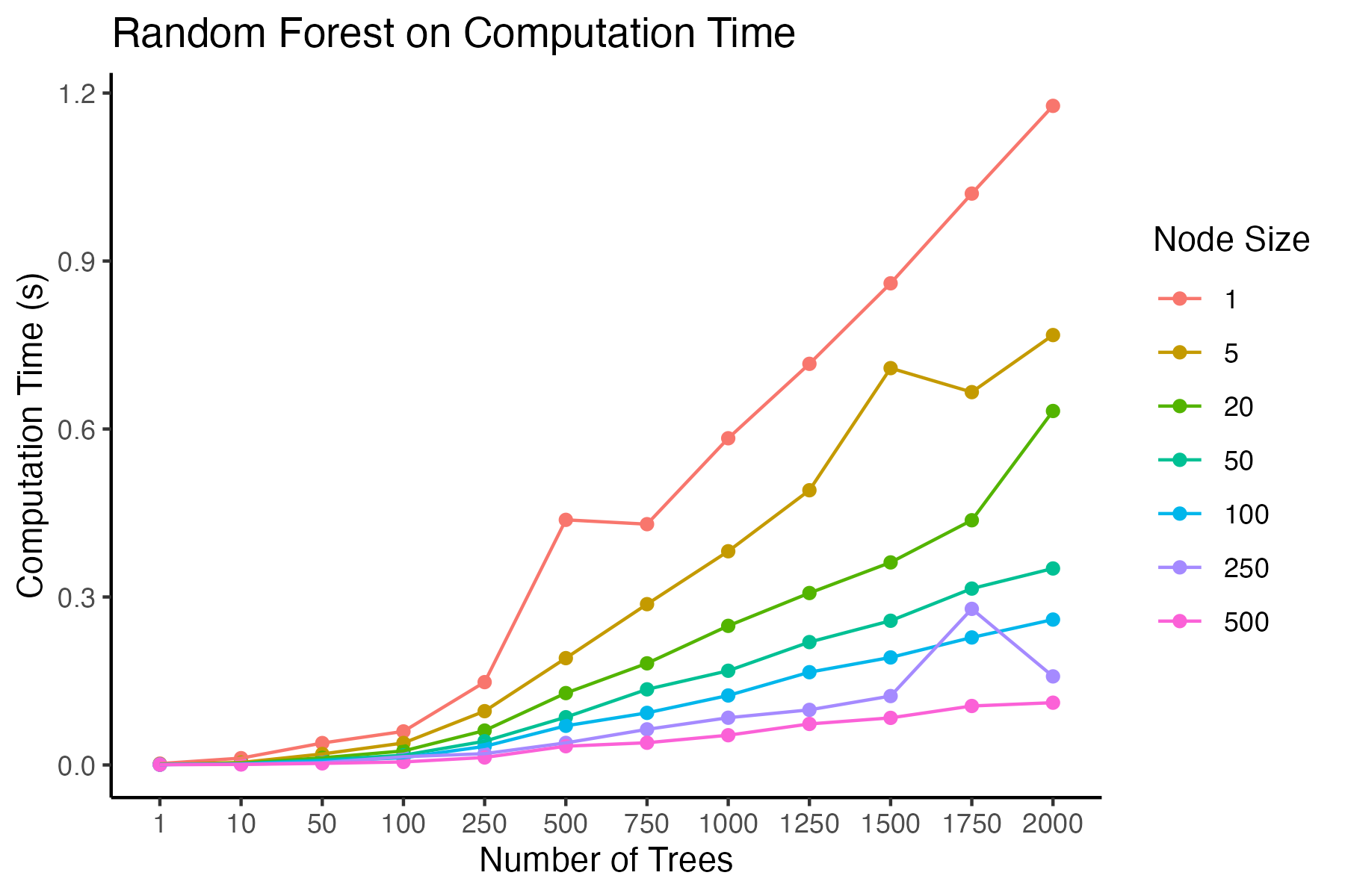
The following graph reveals the recorded computation time to fit a random forest model on a dataset of about 600 rows with only one feature. As we increase the number of trees, we see that the computation time increases gradually. Computational effort also increases when we lower the minimum nodesize (leaf) of a tree. The interaction between ntree and nodesize also exacerbates computation time: because a nodesize of 1 creates very complex trees, creating more trees therefore requires more time to fit a model then the same high number of trees under a nodesize of 10, 20, or even higher. Ultimately, this graph reveals how a large number of complex trees forces the computation time to be longer than a few simple trees.
BART
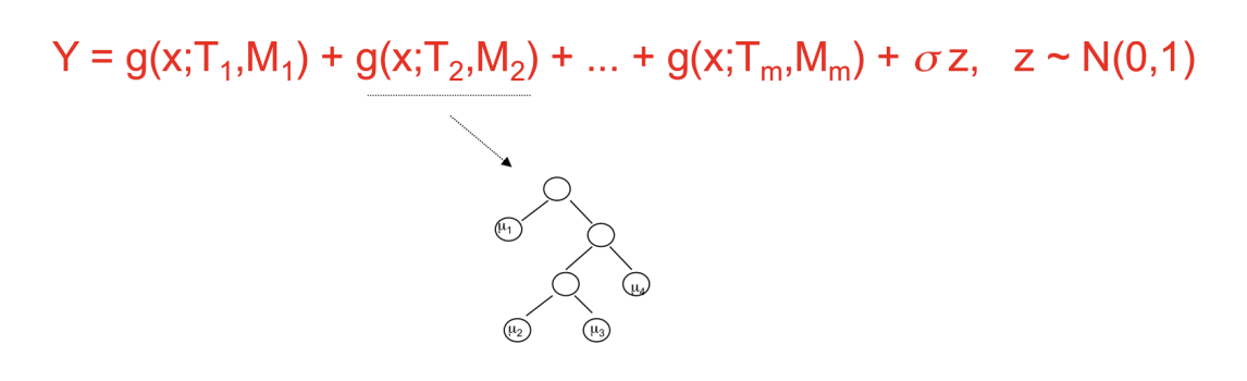
Like random forests, BART also creates multiple trees, but unlike random forests, each tree is heavily constrained to be a weak learner, only meant to cover a particular part of the data. In addition, the ensemble of trees are summed, and not averaged, in regression settings as seen below.
A unique feature of BART is its ability to adjust individual contributions from trees through a Bayesian hierarchal model and imposing priors on the parameters. These priors don’t rely on a metric like the out-of-bag error; rather, the priors control for the complexity of each tree and thus the overall model. This fosters a model that promotes a balance of fit and flexibility, preventing overfit through shrinking the effect of tree contributions towards zero (thus, contributes to the meaning of “a weak learner”).
BART has the ability to assume a prior “tree” distribution and sample random “draws” from this distribution. The “tree” distribution is influenced by parameters that construct the framework of each tree. Each decision tree, as explained with random forests, have certain features that dictate its complexity, such as the branching, node/leaf values, sample representation for each leaf, etc. The “draws” stem from BART being an MCMC Bayesian procedure, meaning that the model will iteratively select a new set of trees. The draws of trees vary in complexity and structure, as well as what parts of the data are strongest or loosely fit. Since each draw provides a set of trees to generate predictions upon, machine learning scientists have a unique option to either use the means of predictions from each set, or to treat each prediction as a posterior predictive distribution. Hence, BART allows Bayesian inference techniques, such as credible (probability) intervals, to become possible for analysis.
Tuning Parameters
The tuning parameters in BART are quite lengthy, but I will focus on these few:
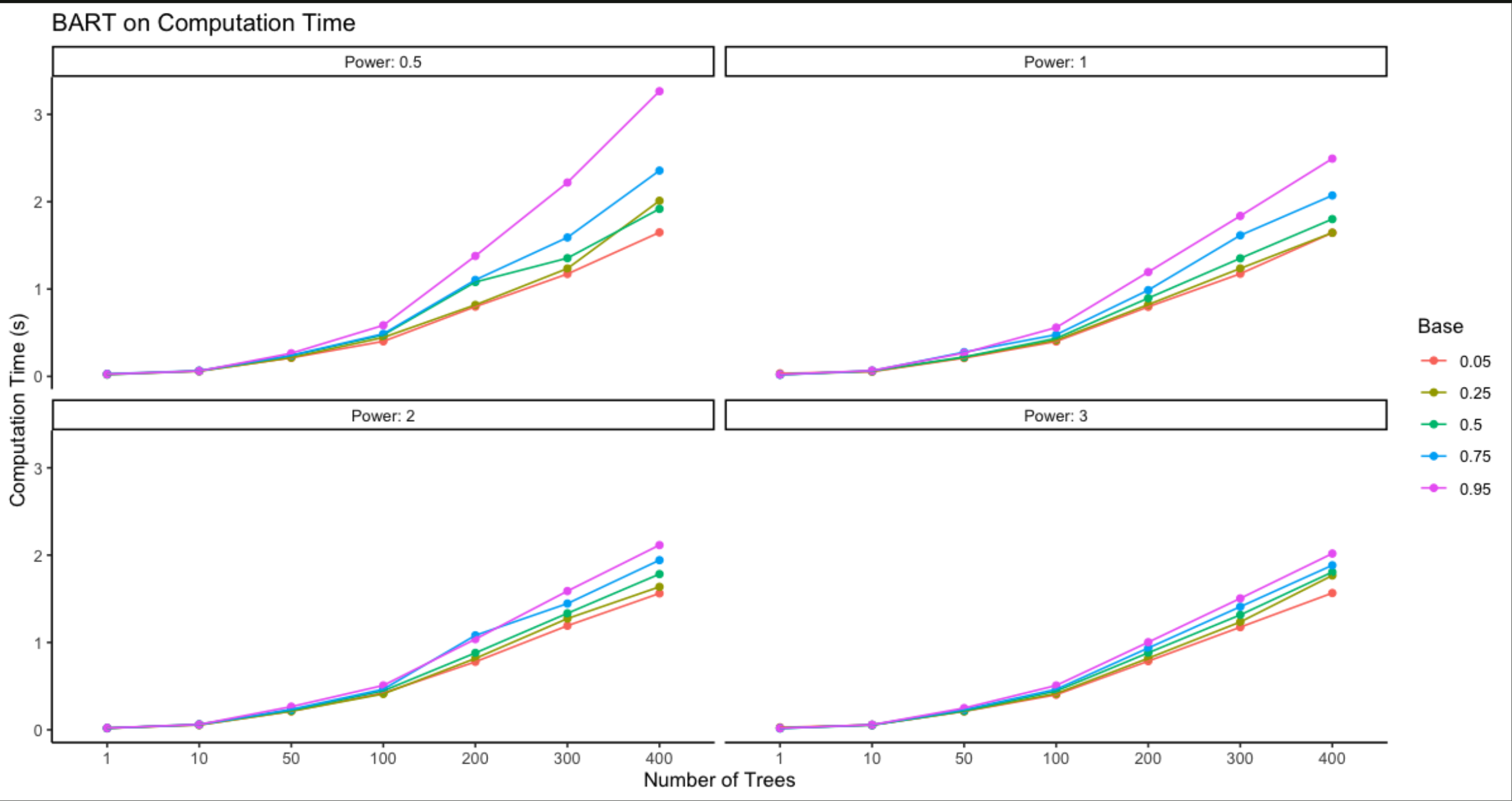
ntreeslike RF determine the number of trees in the model. Each tree contributes to an added sum (instead of mean, unlike RF).baseprior value parameter determining the likelihood a node/leaf splits.powerprior value parameter altering probability of split as depth of tree increases.kprior value parameter that determines the number of standard deviations equal to half the range of the response (i.e. the median of y to the extreme ofkstandard deviations)sigquantprior value parameter that places more weight on fitting noise in data.
For more on the BART model in R, see the following documentation.
Computation Time
Computation time is significantly longer than for random forests. This is due to the iterative sampling BART employs in order to draw multiple sets of trees from a distribution. Certain parameters, such as ntrees, base, power, can exasperate the fitting time for BART, as they require a large quantity or complexity of trees.