Last Updated: 29 Sep 2024
Table of Contents
- Introduction
- Synopsis
- Inference on Monthly Dates and Car Ownership
- Monte Carlo Simulation on Female’s Minimum Height for Male Partner
- Conclusion
Introduction
Last year, I deleted Instagram completely. I was wanting to make a change from my lifestyle where I wasted hours and hours on reels each day. Later in November, however, my family urged me to redownload it and start a fresh profile, looking for more meaningful accounts to follow. That was when I stumbled upon the Instagram profile @UtahStats. With my love of data analytics in the realm of human behavior, psychology, and culture, this profile became a major source of excitement. I would tell my friends to follow this account purely because of how interesting their insights were, and where I think my stats background could help improve the reporting. As I approached the summer of 2024 and an enrollment in a Statistcs masters program at BYU, I wanted to explore more statistical psychology. I reached out to the account owner, Jacob Dunn, purely on a whim, asking if he had a project he would want to collaborate on, or at least have me contribute to. After a couple of discussions, we landed on an idea for a data analytics project with an unpredictable outcome: a summary of his first ever survey.
As a psychology student at BYU, Jacob Dunn had a desire to explore niche facts about college students living in Utah. He learned how statistics can be utilized to study various populations. He created the first “ProvoStats” survey (as it was named then) to collect data, originally passing out fliers to invite students to take the survey and contribute their experiences. Once enough data was collected, Jacob posted unique findings on Instagram. Overtime, the page grew tremendously. As he kept posting more of his findings, Instagram followers demanded more answers to questions about young adult culture. This led to Jacob further enrichening his range of topics by creating multiple surveys with more specialized questions. This opened opportunities for followers from outside Utah County to respond to surveys and contribute to the data, hence creating the brand @UtahStats.
Participants of the @UtahStats surveys are presented with a broad range of questions, and their responses are recorded and processed using Qualtrics. These questions range from topics such as previous relationships, dating, church and college activity, politics, and other topics unique to the Utah County area.
Synopsis
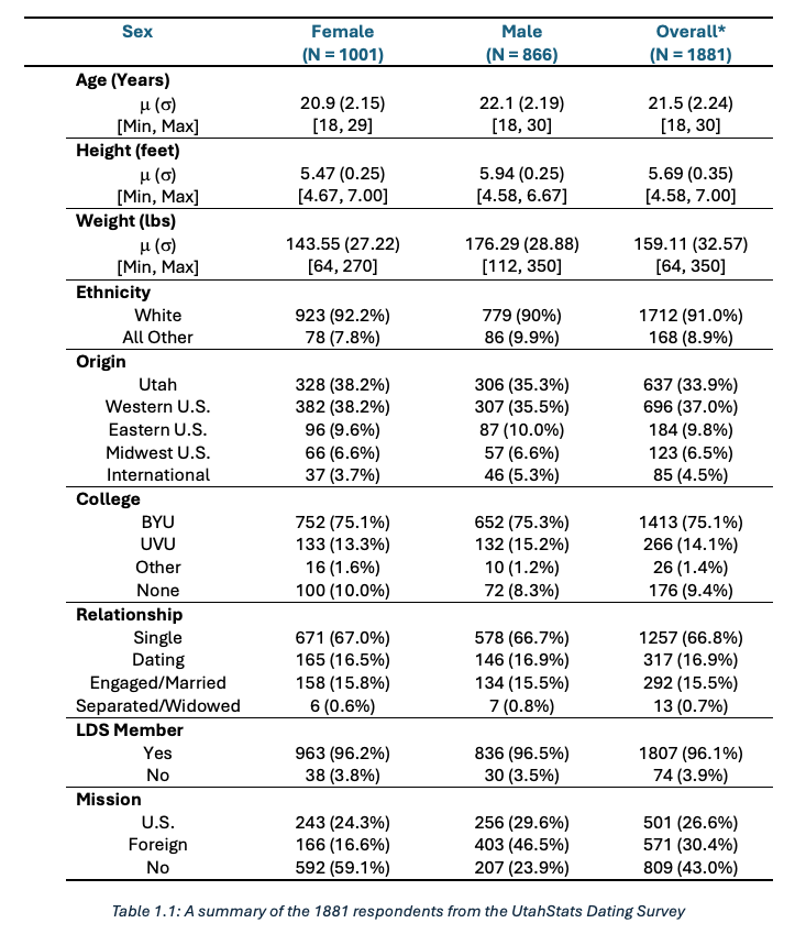
With a sample of 2,101 respondents (and 1,881 had usable data). From our quick exploration of the data and the table 1 below, we understood some of the main characterstics of our sample:
- While the range of our sample covers ages between 18 and 30, 75% are below 23 years of age.
- 75% of survey respondents attend BYU and 14% attend UVU. This emphasizes a geographical response bias towards BYU/Provo young adults being more regular participants than Orem/UVU.
- 96% of survey respondents are of the LDS faith.
- 57% of survey respondents served missions (and 54% of missionaries served in foreign missions).
The next couple sections discuss some of my personal favorites from the paper as they both present some very intersting findings and gave me the opportunity to tap into statistical and technical skills.
Inference on Monthly Dates and Car Ownership
In this figure, we see the effect of car ownership on the number of dates per month. What is astonishing is how different gender and age reacts to car ownership and dating. Apparently, females in this sample under 21 go on significantly more dates when they own a vehicle than females that do not own one (p = 0.004). Males 21 and older who own a car go on significantly more dates than those without a car (p = 1.1e-5).
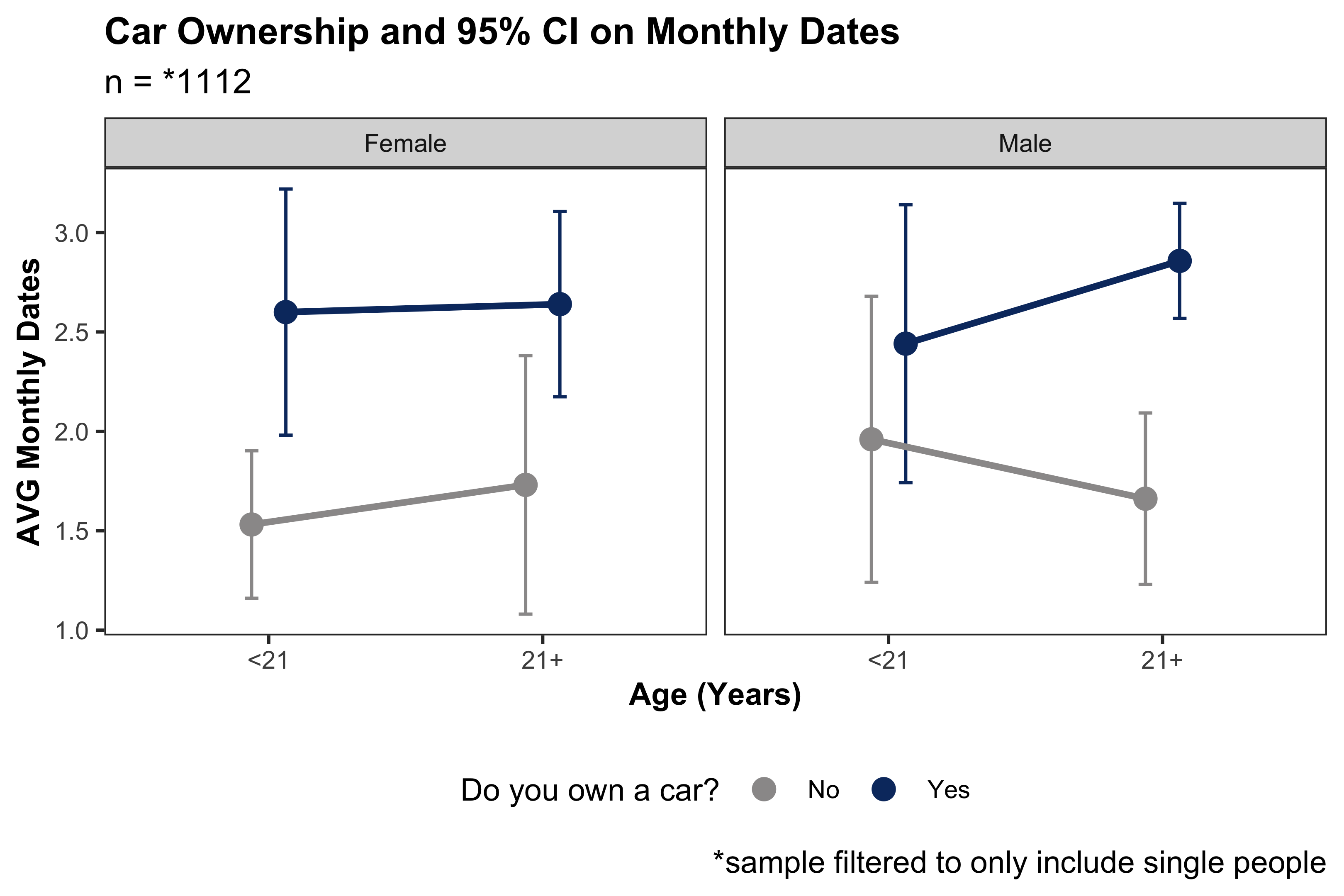
There are a couple of aspects from this analysis I wish to highlight. First of all, I believe this figure teaches a very interesting and convincing story about males 21+. To say and determine that men 21+ in Provo/Orem and whether they own cars is tied to how many dates they can go on in a month can be a fascinating narrative to share in an entertaining research paper. It has viewer shock value, and it is not an impossible situation.
However, the results differ when considering different statistical testing scenarios. There were two tests to consider calculating both intervals and p-values: one was a standard t-test for means among filtered these groups, and the other is t-pairwise comparisons (with a Bonferonni p-value adjustment). The latter, which is not as commonly known among general populations, is considered a more robust approach as it evaluates all group combinations simutaneously while adjusting for Type-I error (i.e. false positives). The t-test can only compare two groups at a time and provides only one p-value and one interval; this ultimately decreases the likelihood of procuring a Type-II error (false negative).
I was left with a difficult decision: if I am interested in reporting potential differences among groups, do I care about reporting false negatives or a false positives? In other scenarios, it depends on the context. For example, if a patient goes in for a cancer screening, a false negative is much more consequential than a false positive, because we would rather administer treatment to someone who does not need care than fail to administer treatment to someone who does. Ultimately, no decision I would be making with this paper would have drastic consequences such as a failed cancer detection test, so I decided to inflate my likelihood of a Type I error (false positive) and utilized two-group t-distribution calculations for this part of the inference.
I only reported testing from the t-test analysis, but I wanted to also see how each the other test compared. As stated already, the p-value for a t-test comparing monthly dates for 21+ year-old males who do and do not own cars was 1.1e-5, which would be considered significant among most decided significance cut-offs. When computing pairwise t-testing, however, the p-value was 0.124 (or 0.044 without adjustment) for the specific subset comparing 21+ year-old males.
Ultimately, there are certainly much better ways to analyze this problem than the one I performed. But this part of the inference, particularly the decision-making on what exactly I report, taught me a lot about how versatile statistical reporting can be, as well as, unfortunately, how easily things can be interpreted one way or another. This is one of those unique cases where statistics becomes more of an art than a science.
Monte Carlo Simulation on Female’s Minimum Height for Male Partner
As many understand (and is further proven in Figure 7.7), women value height as an important characteristic for a male to be a suitable romantic partner. This may be because women report experiencing greater feelings of safety and security when they are around taller men. However, many men feel that women’s expectations for men’s heights is unrealistic. In our survey, we asked the women how tall a man must be to be an eligible partner. We also asked how tall in inches each male was, and used that to assess, based on those heights, how likely women will be able to find a suitable partner. The following work presents a simulation that assesses the height differences between males and females, as well as the height difference they want their partner to be compared to their own. The latter is meant to balance preferences between shorter and taller women.
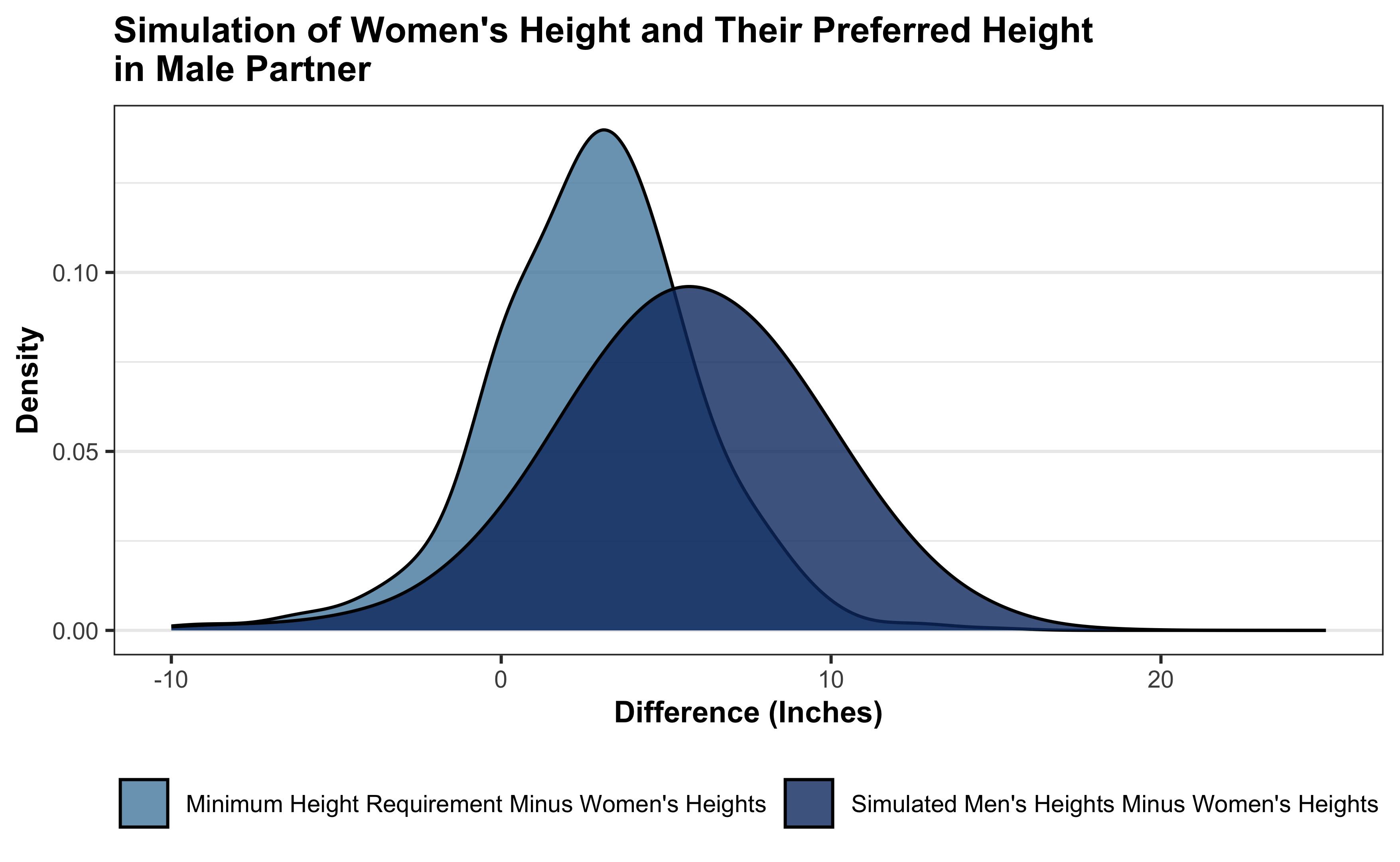
The above figure relays how this simulation plays out. Using the 764 women and 708 men who answered questions regarding height, I created 50,000 “couples” and assessed height differences between men and women. A man is, on average, 5.6 inches taller than their female partner (and thus men are about 8.5% taller than woman, on par with the North American average). This measurement is promising since the preference for women is a man that is on average 2.75 inches taller than them.
This blog serves for me what the paper’s scope cannot take time to cover. It became my first project using a Monte Carlo simulation. The main premise of Monte Carlo is to take random values within a given distribution $X$, and estimate certain statistics such as the mean and standard deviation from a new distribution created from random values. This particular practice helped me find a new distribution resulting from the expected difference between two other distributions – the heights of males, and the heights of females – from the survey. This would then create for me a distribution of heights $X_m - X_f$ that represents the expected difference in randomly paired couples (males - females). And, with the random draws from this created new distribution, I can calculate the probability, or the density, where the new distribution is less than 0 with really simple code.
In the code snippet below, I resampled 50,000 males and females and estimated not just $X_m - X_f$, but also $X_m - X_{pm}$, which is the different between men’s heights and the preferred men’s heights by women.
# Monte Carlo Simulation: potential height differences and preferences between males and females #
n <- 50000 # number of couples to make

sample_female <- female_data[sample(x = 1:nrow(female_data), size = n, replace = T),]
sample_male <- sample(x = male_data$height, size = n, replace = T)
height_differences <- sample_male - sample_female$height
height_requirements <- sample_male - sample_female$height_requirement

# Monte Carlo Insights #
mean(height_differences < 0)
sd(sample_diffs < 0) / sqrt(n)
# 7% of women may find a randomly assigned male partner at least an inch shorter than her
# MC Error: 0.1%

mean(sample_reqs < 0)
sd(sample_reqs < 0) / sqrt(n)
# 20% of women will not find a randomly assigned man that meets their height requirements
# MC Error: 0.2%
If we assumed that $X_m$ and $X_f$ were normally distributed, we certainly could have calculated expected differences such that $E(X_d) = E(X_m) - E(X_f)$ and $Var(X_d) = Var(X_m) + Var(X_f)$ and gotten the same estimates of the distribution of differences. However, when calculating probabilities (like $P(X_d < 0)$), we would fail to accomodate for the fact that our study can only account for differences in heights in inches, and not any values in between (i.e. our simulated distribution is discrete, which is what the form of our data is). This would result in different probabilities yielded. Also, doing simulations in a paper sounds so much cooler! We then report the following Monte Carlo estimates from the code above.
Overall, this sounds like the women in our survey have reasonable and logical expectations for the minimum height requirement for men. In this simulation, only 7% of our randomly matchmade couples had the man shorter than the woman, and only 20% of women were paired with someone that did not meet their minimum height requirement. That means that generally, women in the Provo/Orem area hold preferences for men’s heights that are very reasonable to the men available.
Conclusion
I learned a lot about how to report statistical inference with many complications in statistical reasoning in mind, namely survey response biases, imbalanced groups, and reporting findings under the pretense of a generally non-academic audience and doing so with statistical cautions in place. I also explored how different statistical methods have pros and cons, such as how Type I and Type II inflation influences p-values, and how Monte Carlo simulations can be used to expand questions from real-world data. Finally, the experience taught me how to tell a compelling story using visualizations, tables, and modeling in context of young adult dating culture, which is a very unique and interesting topic to report statistics on.
If you want to learn more about my statistics work on this project, I recommend checking out the full PDF! It is only $5, and can either be a very insightful deep reading, or a fun document to skim through. Either way, any support you offer me will help create more reports like this in the future!
You can view the PDF here.