Last Updated: 26 Oct 2024
Table of Contents
Abstract
This study explored how different coaching cues impacted 39 young athletes’ performance on a single-leg triple hop test. Specifically, internal cues (focusing on body movements) and external cues (focusing on an object beyond their reach). Each athlete completed three practice trials before receiving instruction relevant to their group. Those in the internal cue group received coaching emphasizing arm movements, while the external cue group was told to aim beyond a cone. The control group watched a video that was unrelated. Performance was measured by the change in jump distance from before to after receiving the cues, with angles at the hip, knee, and ankle analyzed using motion capture.
Univariate ANOVA results showed that the external cue group had significantly greater improvements in jump distance than both the control (by 8.3%) and internal cue (by 7.1%) groups (p = 0.0059 and p = 0.0148, respectively). These improvements were similar for both males and females. Additionally, secondary findings revealed moderate correlations between changes in joint angles, particularly the ankle and knee (r = 0.70). The study suggests that using external cues could be a promising coaching approach to boost performance and potentially reduce injury risk in young athletes. Multivariate ANOVA (MANOVA) infers that groups overall kinematics among treatment groups also differed (p = 0.004), particularly pairwise comparisons between external and interal cues (p = 0.010) and potentially between external and control (p = 0.071).
Introduction
BYU sponsors its Exercise Science program, its faculty, and select students, to host the (Strong Youth Project)[https://exsc.byu.edu/the-strong-youth-project-homepage] (SYP), with its focus to promote positive experiences in sports for youth. Encouraging children’s sports fights health concerns like obesity, diabetes, depression, and other common challenges in society. With a focus on implementing evidence-based insights in athletic performance, SYP sponsors various projects for both children and youth coaches to benefit from.
The SYP team reached out to many other departments to participate and develop their research, one of which was the statistics department. My professor and I were called in to analyze a dataset related to different youths’ reception to training cues, particularly for an exercise called the single-leg triple-hop. As demonstrated in the video below, the subject is to jump as far as they can in three jumps using one leg of their choice. Motion capture technology, called OpenCap, videos each subject and renders a 3D frame of their body. It also calculates metrics based on their kinematics (that are important to our study), including their hip, knee, and ankle angles, and the amount of time their foot is on the ground between jumps (called stance time). The experiment included three types of treatments, or coaching cues, to teach the youth: a video unrelated to the exercise (control), a training demonstration on good jumping form (internal), and an object to jump too that was beyond their reach (external).
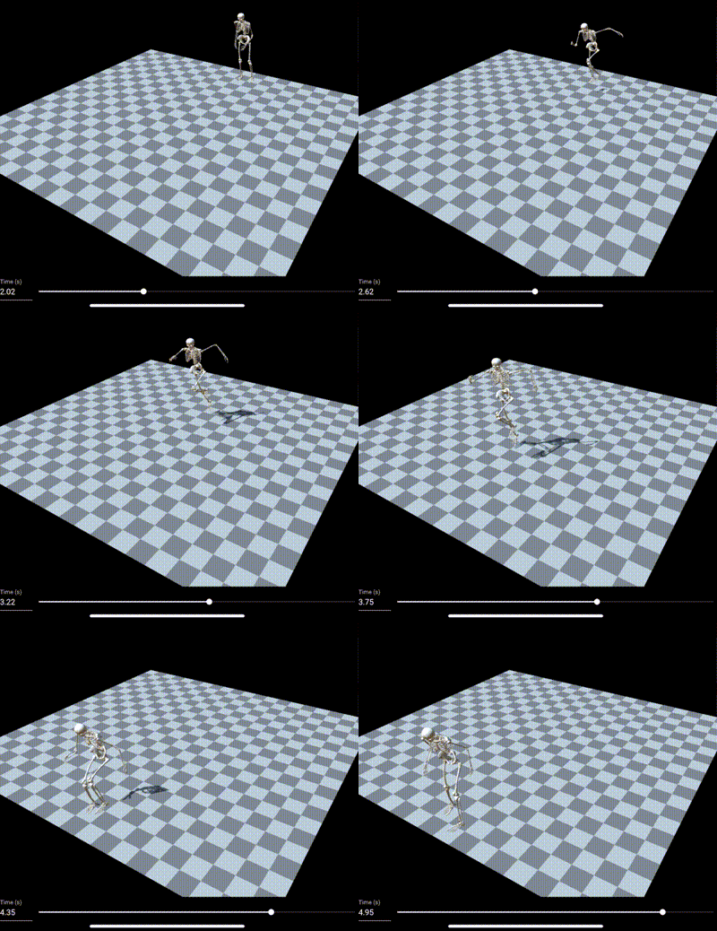
This analysis aims to answer the following questions related to the triple-hop experiment:
- Do the three different coaching cues differ in triple-hop jumping distances?
- Do the three different coaching cues influence jumping techniques (kinematics)?
- What is the relationship between coaching cues and changes in kinematics?
Methods and Results
It is important to note too that this case will be considering five separate variables in the forms of percent change, namely the jump distance, ankle, hip, and knee angle changes, and the stance time. That means I had to learn and explore different multivariate methods. My process of working through this data was by first exploring the data itself (EDA), and following that then performed univariate ANOVA, multivariate ANOVA, and LDA (also known as linear discriminant analysis), with the latter two being more unfamiliar to me at this point in my education.
EDA
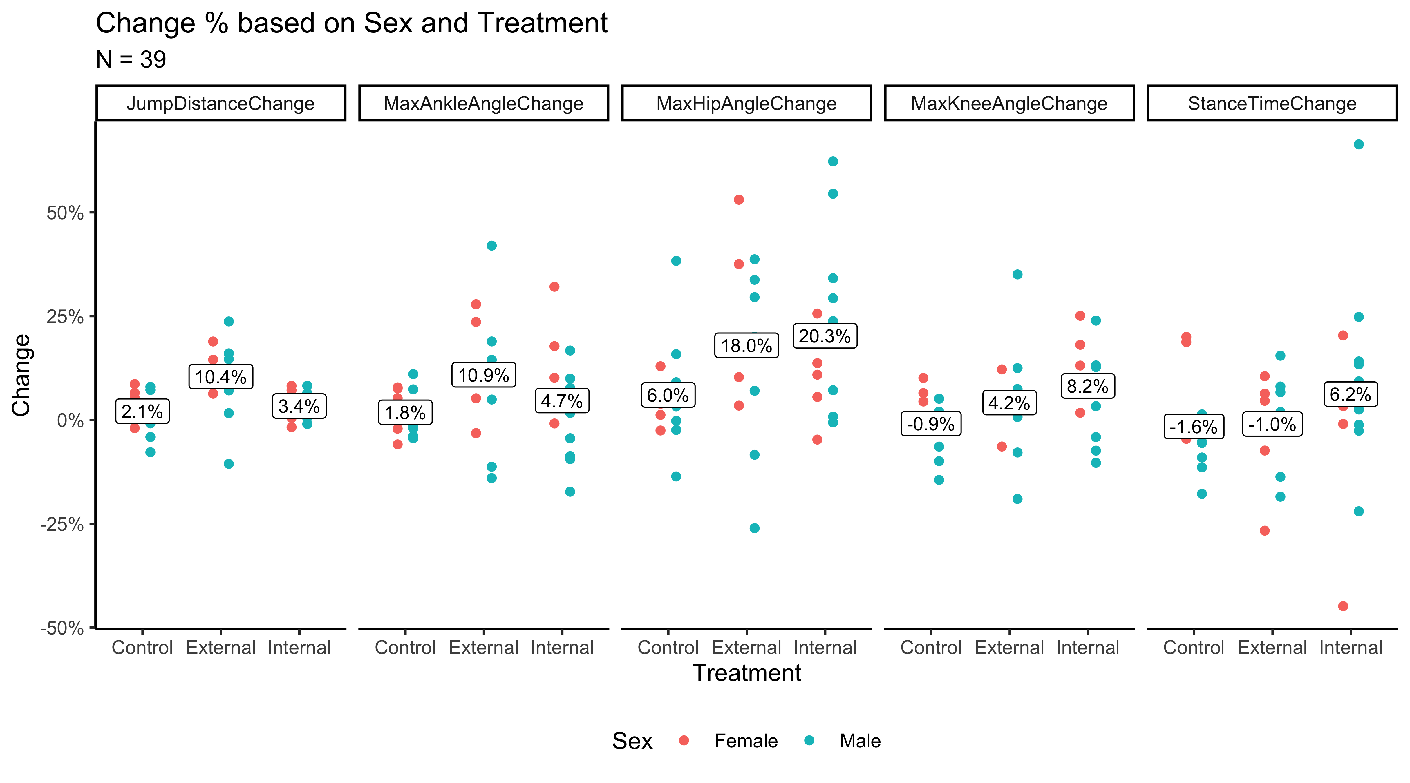
The following figure below visualizes how each variable of percent change differed among treatment groups. Notably, we see that the external group had an average 10.4% jump distance increase, compared to the control at 2.1% and internal at 3.4%. This was a promising indicator that external training seems to influence the participants’ abilities to jump further than they previously could: in sports performance, a 10% increase in any exercise is certainly impressive. When also visualizing ankle, hip, knee, and stance time, we could also make visual inference about group differences here, but notice how varied each point is. These variables tended to be much more volatile than jump distance, which may make significance among treatment groups harder to detect.
To answer questions about each variable influence amongst each other, I also explored creating a correlation matrix among each of the response variables, as seen below. I find correlation matrices a popular tool for understanding data quick (assuming these variables are continuous and linear). Also, correlations are typically widely understood among many, including the exercise science team, and so demonstrating this graphic really excited them.
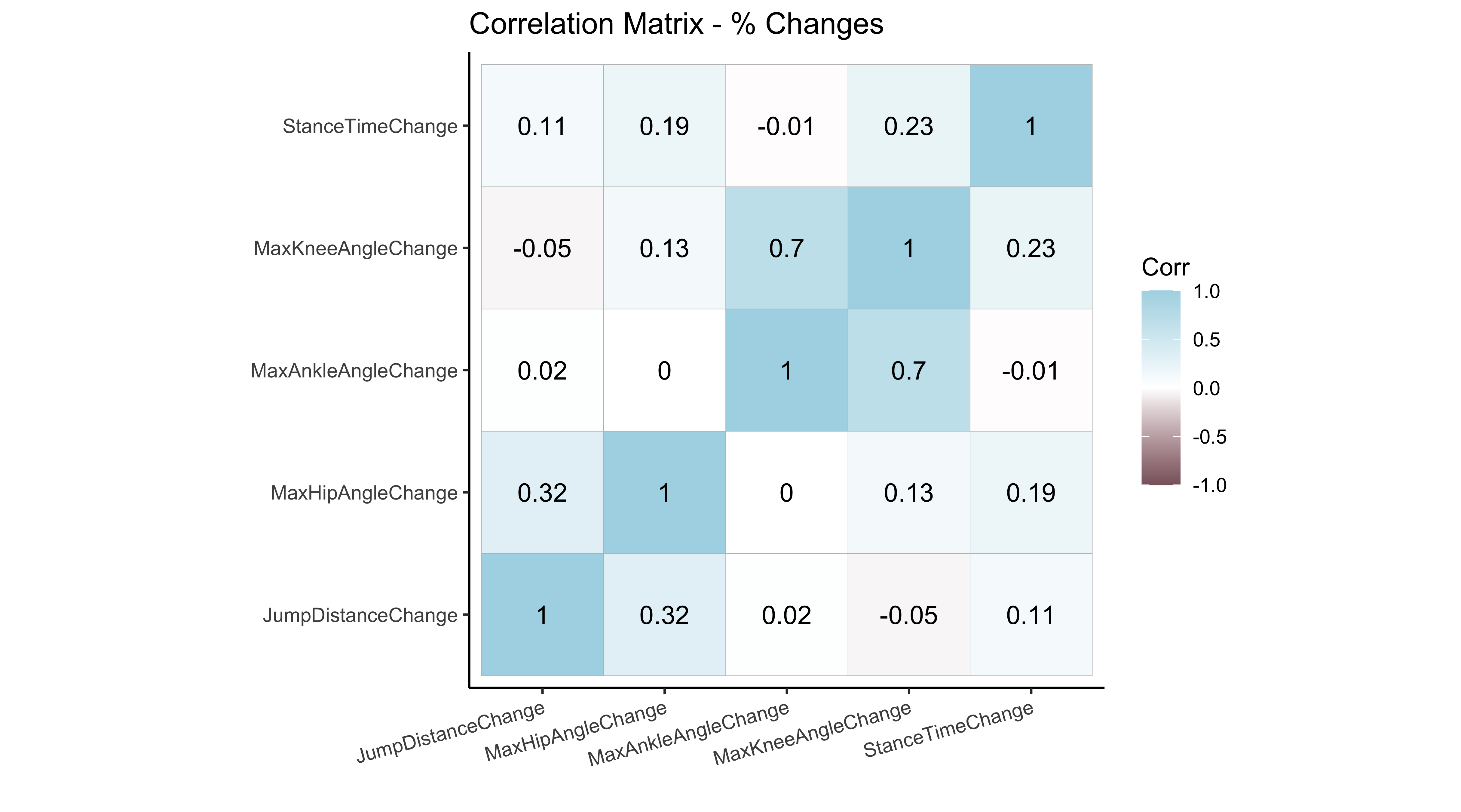
I promise I am not overstating this when I say that when I showed the correlation matrix to them, they stared and discussed it for 15 minutes. Not that it was confusing, but the first time they’ve been able to see how kinematics related to each other. They also started discussing theories among three angle connections related to anatomy that are beyond topics that I know, but it was very interesting to see how they connected my data analysis to their field of study so cleanly – all of it was amazing to sit in and experience. One of these theories that circulated and finding were about the strong 0.70 correlation between knee and ankle angle, specifically how diving down into a deeper stance in your knee also flexes your ankle drive more. In addition, the hip angle with a mild correlation of 0.32 may relate to how deeper hip flexion drives your jump distance a little bit more.
I share these because sometimes statistical analysis may get data scientists, statisticians, and like-groups excited, but for other backgrounds, they get lost or bored quickly. Using data visualization to introduce statistical findings is an important tool to excite audiences about the power of using analysis methods.
ANOVA
This section aims to answer how the coaching cues differ with jump distance purely. As noted already, the external group had a 10.4% change in jump distance, which was 8.3% higher than the control group and 7.1% higher than the internal group.
The ANOVA method determines differences among group means, and as such, determined that treatment indeed was significant (p = 0.005). The ANOVA also considered other variables that we don’t discuss fully in this blog, namely sex, the initial jump distance, a treatment-sex interaction term, and a sex-initial jump distance interaction term. The ANOVA component of this code is featured below in R. None of these terms were considered significant, but they do help control for potential bias and answer some of our sub-questions.
lm_jump <- lm(JumpDistanceChange ~ Treatment*Sex + Sex*AVGPreJumpDistance, data = syp)
# note that * uses the first term, then the second, then the interaction.
anv_jump <- anova(lm_jump)
print(anv_jump) # treatment at p = .005
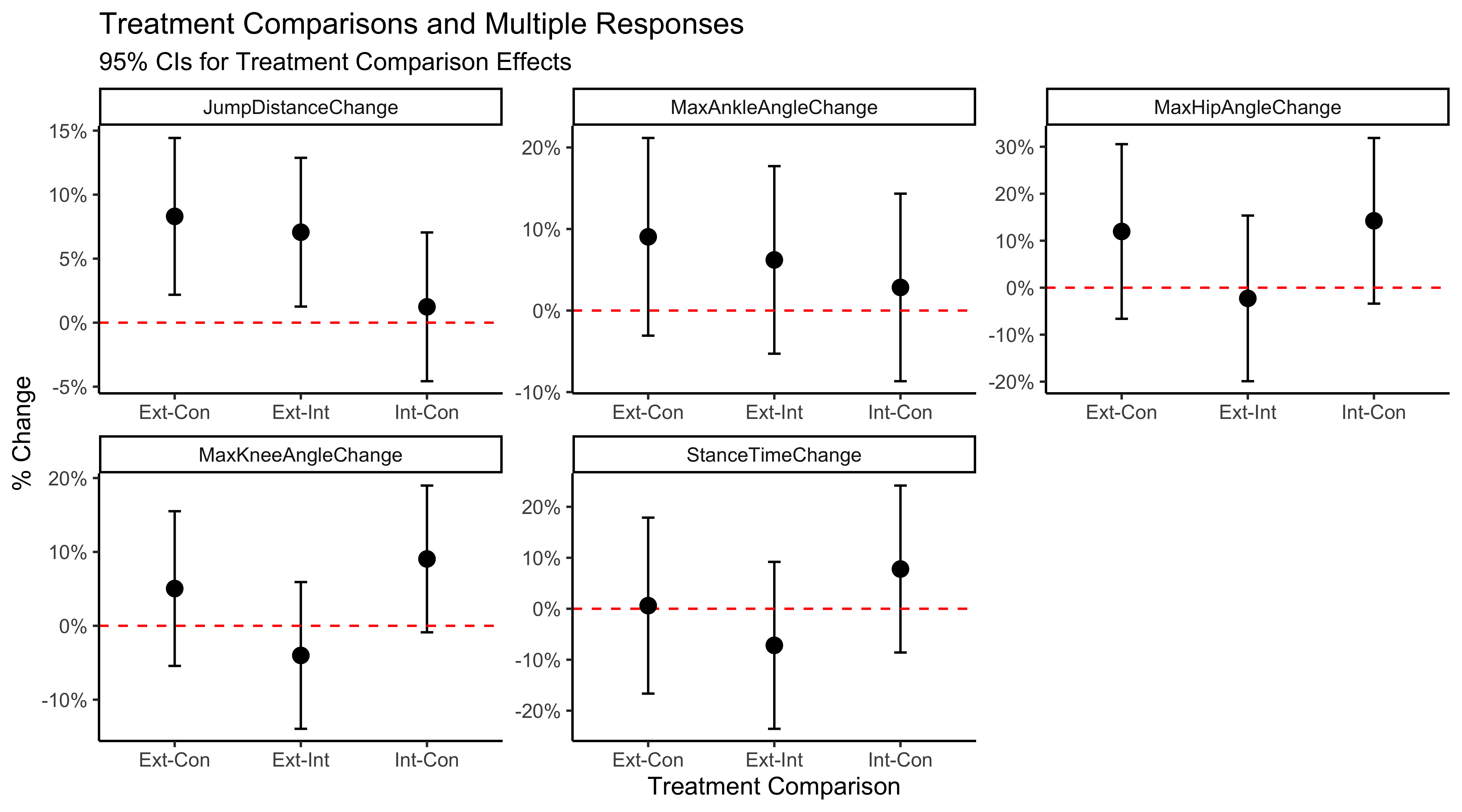
In addition, we are interesting in doing pairwise comparisons among treatment groups. This will tell us about the effect of one treatment group and how it differs to another. TukeyHSD() is a great function for computing these pairwise differences. The graph below essentially calculates these pairwise differences (for all variables of interest), and reveals how some of these comparisons hang above the zero line, indicating treatment effects among group. With a bonferroni p-value adjustment, the external-internal and external-control pairwise comparisons are significant (p = 0.0059 and p = 0.0148). Internal-control is not significantly different (p = 1). Note that I did the pairwise comparisons for all groups, but only jump distance has significant comparisons above zero.
MANOVA
Like ANOVA, MANOVA is a statistical technique for analyzing differences between groups when there are multiple dependent variables. Conducting separate ANOVAs on multiple dependent variables can increase the chance of false positives (Type I errors). MANOVA simultaneously considers all performance metrics, including the four kinematics variables along with jump distance, how how they collectively respond to the external, internal, and control groups.
Our analysis using MANOVA concluded an overall significance among jump performance and kinematics for the treatment group (p = 0.004). Like our ANOVA analysis, sex, initial jump distance, treatment-sex interaction term, and the sex-initial jump distance interaction term were all non-significant.
mva <- manova(cbind(JumpDistanceChange, MaxHipAngleChange, MaxAnkleAngleChange, MaxKneeAngleChange, StanceTimeChange) ~
        Treatment*Sex + Sex*AVGPreJumpDistance, data = syp)
print(mva) #treatment p = 0.004
We also found the pairwise comparisons among the multivariate setting, but this is only useful for interpreting group-by-group significance. Accordingly, the external-internal comparison was significant under a Bonferonni adjustment (p = 0.011), but not for external-control (p = 0.071). The internal-control difference was also non-significant (p = 0.395).
LDA
MANOVA, while useful in determining whether there are overall differences among groups, doesn’t specify which individual variables are influenced by each treatment group. Linear Discriminant Analysis (LDA) becomes valuable here because it allows us to identify specific variables and their contributions to group separation. LDA can provide:
- A transformation of the data that maximizes group separation by finding linear combinations of predictor (independent) variables (which are interval or ratio) to predict categorical group membership, essentially reversing the ANOVA and MANOVA framework by focusing on predicting group categorization.
- Insight into which components of the predictor variables (e.g., kinematics and jump distance) contribute most to the discrimination among treatment groups, making it possible to pinpoint the factors that drive differences.
- Quantification of the change associated with each variable, illustrating how much each contributes to distinguishing between groups, which is helpful in understanding relative importance and the nature of variable relationships across groups.
Given an input matrix $X$ and a grouping variable, we calculate the within-group covariance matrix $E$ and the between-group covariance matrix $H$.
-
Calculate the group means for each of the $k$ groups: \(\begin{align*} \bar{x}_i &= \frac{1}{n_i} \sum_{j \in \text{group } i} X_j \end{align*}\) where $n_i$ is the number of observations in group $i$, and $\bar{x}_i$ is the mean vector for group $i$.
-
Compute the grand mean $\bar{x}_{\text{all}}$ across all groups: \(\begin{align*} \bar{x}_{\text{all}} &= \frac{1}{n} \sum_{j=1}^{n} X_j \end{align*}\)
-
Calculate the within-group covariance matrix $E$: \(\begin{align*} E &= \sum_{i=1}^{k} \sum_{j \in \text{group } i} (X_j - \bar{x}_i)(X_j - \bar{x}_i)^T \end{align*}\)
-
Calculate the between-group covariance matrix $H$: \(\begin{align*} H &= \sum_{i=1}^{k} n_i (\bar{x}_i - \bar{x}_{\text{all}})(\bar{x}_i - \bar{x}_{\text{all}})^T \end{align*}\)
Step 2: Eigen Decomposition and Discriminant Function
-
Perform eigen decomposition on $E^{-1/2} H E^{-1/2}$ to obtain eigenvalues and eigenvectors: \(\begin{align*} C &= \text{eigen}(E^{-1/2} H E^{-1/2}) \end{align*}\)
-
Form matrix $D$, the matrix of discriminant function coefficients: \(\begin{align*} D &= E^{-1/2} C_{\text{vectors}} \end{align*}\)
-
Standardize $D$: \(\begin{align*} D^* &= \text{diag}(\sqrt{\text{diag}(E)}) \times D \end{align*}\)
Step 3: Calculate Discriminant Scores
Using $D^*$, calculate the first and second discriminant scores, $z_1$ and $z_2$, by projecting $X$ onto the columns of $D$: \(\begin{align*} Z &= XD \\ \end{align*}\)
The 5x5 $D$ matrix represents the standardized coefficients of the linear discriminant functions. It also allows us to understand the relative contributions of each variable to the discriminant functions. Each column of $D^*$ corresponds to a discriminant function, and the elements indicate the strength and direction of each predictor’s contribution. Conversely, the 39x5 $Z$ matrix contains the discriminant scores calculated by projecting the original data matrix $X$ onto the discriminant function coefficients in $D$. The scores $z_1$ and $z_2$ provide a way to visualize and interpret the separation of groups based on the linear combinations of the predictor variables. By plotting $Z$, By plotting $Z$, we can visually assess how well the groups are separated in the multivariate space. The closer the points of different groups are to each other, the less separable the groups are, while greater distances indicate better separation. From our MANOVA results, we should see this group separation at play.
The figure below demonstrates how the treatment groups of external (green), internal (blue), and control (red) are separable in the discriminant space. The interesting insights from this graphic is first noticing the density plots of $z_1$ for each cue (top left). The green external group has more positive $z_1$ scores than red control and blue internal, which are highly populated towards lower scores. Conversely, we see $z_2$ scores separate blue internal from red control (bottom left). Each of the scatter plots (on the top right and bottom left) portray the dimension-reduced clusters of each cue. We note that $z_1$ does the best job separating the treatment groups with the external to the far right (if looking at the bottom left plot), with its eigenvalue determining this as explaining 67% of the Z-space variance. $z_2$ than is separating internal and control in that space with explaining a remaining 27% of variance.
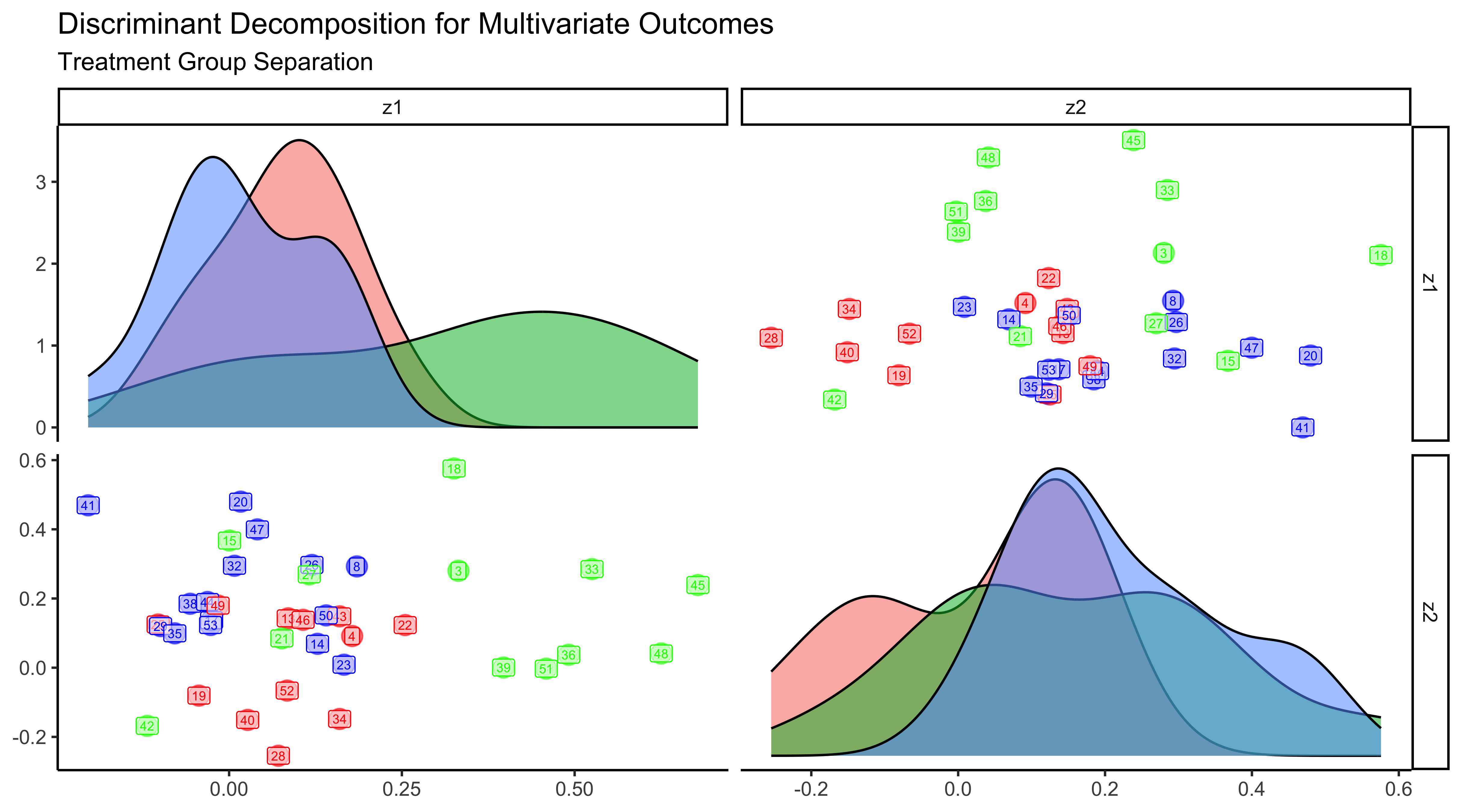
The clustered data visualization makes the discriminant functions $D_1^$ and $D_2^$ much more interpretable. When we examine the coefficients of the discriminant functions associated with each variable, they indicate the relative influence of each variable in distinguishing between treatment groups. Values farther from zero signify greater influence; thus, coefficients with larger absolute values contribute more significantly to the discriminative power.
For instance, in the $D_1^*$ function, the jump distance, ankle angle, and knee angle have particularly large magnitudes, suggesting that these variables show significant changes under the external cue condition. Specifically, the coefficients for jump distance (0.85) and ankle angle (0.98) indicate that these variables are more responsive to the external cue compared to the knee angle (−0.71), which also shows notable sensitivity.
\[\begin{equation*} \mathbf{D_1^*} = \begin{pmatrix} \text{Jump Distance} \\ \text{Hip Angle} \\ \text{Ankle Angle} \\ \text{Knee Angle} \\ \text{Stance Time} \end{pmatrix} = \begin{pmatrix} \textbf{0.85} \\ -0.11 \\ \textbf{0.98} \\ \textbf{-0.71} \\ -0.17 \end{pmatrix} \end{equation*}\]The second discriminant function $D_2^*$ indicates that hip angle (.52) and knee angle (.95) have greater discriminatory power for the internal group compared to the control group. This may indicate how the internal cue participants received instruction on deeper hips and knee drive, but ultimately did not influence their jump performance.
\[\begin{equation*} \mathbf{D_2^*} = \begin{pmatrix} \text{Jump Distance} \\ \text{Hip Angle} \\ \text{Ankle Angle} \\ \text{Knee Angle} \\ \text{Stance Time} \end{pmatrix} = \begin{pmatrix} 0.25 \\ \textbf{0.52} \\ -0.34 \\ \textbf{0.95} \\ 0.03 \end{pmatrix} \end{equation*}\]Conclusion
In conclusion, this project successfully showcased several advanced statistical analysis techniques tailored for multivariate analysis, allowing us to delve deeper into our research questions. Through ANOVA, we not only confirmed significant improvements in jump performance attributable to the external cue but also employed MANOVA to demonstrate that biomechanical variables varied significantly across treatment groups. Furthermore, using Linear Discriminant Analysis (LDA), we identified how these kinematic differences influenced group classification and their interrelationships. This comprehensive approach not only enhances our understanding of the data but also establishes a robust framework for future studies exploring the effects of various cues on performance metrics.
The full project was featured in a couple places too!
- Article on SYP
- Instagram post (notice a familiar graphic?)
- Youtube Video (view 10:30 through 13:20)
- Academic paper pending.