Last Updated: 07 Jan 2025
Table of Contents
Abstract
Raw data frequently comes in with multiple errors, including some cells of a dataframe being missing. The following project evaluates the varying processes and algorithms that attempt to handle this concern, aiming to either remove the rows with missing data, or attempting to replace them with a best-guess approach. The following project aims to synthesize three different methods and how they handle missing data, namely List-Wise Deletion, Expectation Maximization, and Conditional Sampling. We perform a Monte Carlo simulation study to simulate various multivariate normal (MVN) distributions with varying correlation structures and patterns of missing data (MCAR, MAR, and MNAR). Regarding the latter, we utilized Little’s MCAR test as a simplistic method to determine the missing data patterns. The simulation study provides the backbone of how each method retains the mean, variance, covariance, and correlations of the original dataframe. Finally, the study results indicate that Expectation Maximization performs best under these scenarios, favoring both an accurate approximation of the data parameters with the best precision. Future studies could expand upon the current project layout to determine how EM (and other methods) perform under different multivariate distributions.
Introduction
Raw data is commonly riddled with errors. A consistent challenge for statisticians, machine learning engineers, business analysts, and other professions specializing in data modeling is to to determine the best approach for cleaning data. Sometimes this objective comes with a decision to determine how to handle missing values in data.
As frequent of a circumstance for observing missingness in data is for a data specialist, it quickly becomes problematic for fitting models. Some quick and efficient methods include filling the missing cells with the most frequent observation, the mean or median value, or the cell value from the previous or next row. However, these quick and computationally inexpensive imputation methods fail to consider variable relationships and can blur correlations (which are sometimes necessary for a quality model). Another method is to simply drop the rows with a missing cell or cells, but this route truncates the amount of usable data for modeling and does not guarantee that the covariance is maintained.
This latter consequence is due to different types of missingness. For the researchers collecting data, the inability to observe a particular value may stem from certain conditions, meaning it proved difficult to measure or too extreme of a measurement to record. For the scope of this research paper, we will consider three types of missing data:
- MCAR (Missing Completely at Random): When missing observations are completely random and have no pattern. The probability of being missing is the same for all cases.
- MAR (Missing at Random): When the missing versus observed observations are no longer coming from the same distribution. The probability of being missing is dependent upon other known values within the data.
- MNAR (Missing Not at Random): When missing values within a dataset are due to uncontrollable circumstances. The probability of being missing is related to its own value.
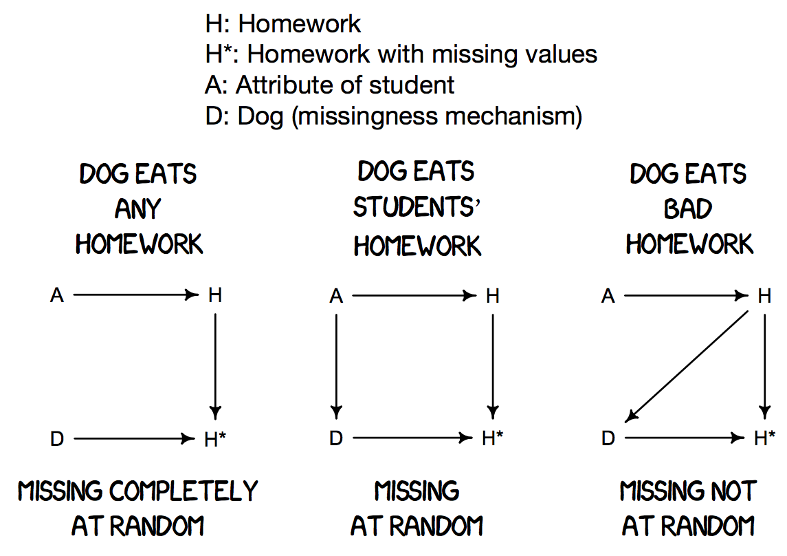
This project will explore, evaluate, and contrast three imputation methods for handling missing data: List-Wise Deletion (LWD), Expectation Maximization (EM), and Conditional Sampling (CS). The analysis will then focus on their computational procedures, strengths and weaknesses, and performance under MCAR, MAR, and MNAR scenarios. We will use a simulation study to generate datasets from a multivariate normal distribution (MVN), varying the mechanism of how the values become empty. The study will evaluate each method’s ability to capture the true mean, variance, covariance, and correlation from its imputed values. The simulation will also use a method called Little’s MCAR Test that can classify the type of missing data. We will end with an outlook on extensions for further imputation method research, as well as connections for an outlier detection algorithm to be developed.
Methodology
The three imputation methods List-Wise Deletion (LWD), Expectation Maximization (EM), and Conditional Sampling (CS) handle missing data with varied approaches.
List-Wise Deletion
List-Wise Deletion (LWD) is the simplest method of the three. LWD removes any observation with at least one missing value, effectively reducing the dataset to complete cases. For our study, LWD will serve as the “control” algorithm. LWD is simply:
\[X_{\text{complete}} = \{x_i \in X_{\text{observed}} : \forall j, x_{ij} \neq \text{NA}\}\]The strengths in the above process lies in its efficiency, with it being a very accessible, quick, and an intuitive function in common data analyst programming languages (e.g. na.omit() in R and pd.dropna() in Python’s Pandas).
clean_data <- drop_na(na_data)
However, sacrificing the sample size and keeping only the complete data is forfeiting valuable information otherwise very useful in a machine learning model or decreasing the amount of uncertainty in an inferential analysis. In addition, LWD is not void of bias: when cells from one column are missing due to the observed values from other columns (i.e. MAR or MNAR), LWD opts to drop that information as well, ultimately cutting out valuable information from that variable’s distribution.
Expectation Maximization
Expectation Maximization is a computationally powerful method that iteratively ‘guesses’ on the missing data while maximizing the likelihood estimation of that guess, based on the observed data. EM alternates between estimating the expected values of the missing data given current parameter estimates (Expectation-step)…
\[Q(\theta|\theta^{(t)}) = E(logL(X_{\text{complete}}|\theta)|(X_{\text{observed}},\theta^{(t)}))\]…and then updating the parameter estimates to maximize the likelihood of the complete data (Maximization-step).
\[\theta^{(t+1)} = \operatorname*{argmax}_{\theta}Q(\theta|\theta^{(t)})\]The iterations end when the change in parameter estimates falls below a predefined threshold (usually small, like $1e^{-5}$). Larger thresholds make for quicker convergence but reduced accuracy.
mat <- as.matrix(na_data)
s <- prelim.norm(mat) # preliminary object, identify data patterns with s$r
thetahat <- em.norm(s, criterion = 1e-5, showits = F) # EM algorithm for finding MLEs
rngseed(123) # needs to be run first for imp.norm to work
clean_data <- imp.norm(s, thetahat, mat) # create imputation data
In R’s norm package, the em.norm() function estimates the parameters, and the imp.norm() function imputes missing data based on these estimates.
EM may prove to be particularly effective when handling MAR and MCAR data, as it estimates parameters by leveraging both means and covariances under the assumption of multivariate normality. This approach preserves the covariance structure of the data, which is essential for multivariate analyses. However, EM’s success depends on its ability to converge, which may be impeded by overly complex data, high proportions of missingness, or violations of the normality assumption.
Conditional Sampling
Conditional Sampling (CS) involves generating multiple imputations for missing multivariate data, each conditioned on the observed mean and covariance structure. CS assumes the data follows a MVN distribution and imputes missing values by drawing samples from this distribution. Unlike EM, which iteratively estimates a single set of parameter estimates, CS generates multiple datasets through conditional stochastic sampling such that
\[X_{miss}|X_{observed} \sim N(\mu_{miss|observed}, \Sigma_{miss|observed})\]In R, the mice package can implement CS with method = "norm" and m = 5 to generate five versions of the dataset. Computing multiple imputations reflect uncertainty in the missing data, which can be analyzed collectively using statistical techniques like the pool(). For our study, we will be pooling in a different method by taking the average of the five imputation versions.
impute_data <- mice(na_data, method = "norm", m = 5, printFlag = F) # conditional sampling based on Bayesian framework
impute_data <- complete(impute_data, "all") # extract all m versions
clean_data <- Reduce("+", impute_data) / length(impute_data) # pool imputed cells together
CS is effective for handling both MAR and MCAR data because it considers the joint distribution of the variables, repairing both the mean and covariance structure. This makes CS more robust than LWD, particularly in preserving statistical properties of the data. Two strengths of CS over EM are its inexpensive computation and no reliance on convergence. Instead, multiple imputations are generated directly.
Little’s MCAR Test
Little’s MCAR test utilizes a $\chi^2$ distribution to test the null hypothesis that an incomplete dataset’s missingness mechanism is Missing Completely at Random (MCAR). The test evaluates whether the means of observed variables differ significantly across patterns of missingness. If the group means differ greatly between patterns, then the $\chi^2$ statistic would be larger. The test statistic is calculated as
\(\chi^2 = \sum_{p \in P} \sum_{j \in J} \frac{n_p (\bar{x}_{pj} - \bar{x}_j)^2}{s_j^2}\) where $P$ indicates the different missingness patterns among the $J$ variables/columns.
Larger test statistics and smaller p-values lead to rejecting the null hypothesis and conclude that the missing data is not MCAR. A key limitation of this test is its inability to distinguish between MAR (Missing At Random) and MNAR (Missing Not At Random), as it only assesses whether data satisfies the MCAR assumption. Distinguishing MAR from MNAR requires other methods beyond the scope of this paper.
In this study, Little’s MCAR test will verify whether simulated datasets exhibit MCAR missingness.
Simulation Study Setup
The simulations performed will provide evidence on how each method handles missing data and estimates the statistics of interest. A given simulation will generate a dataset from an MVN distribution, and randomly remove cell values from the data in the form of MCAR, MAR, and MNAR. The best algorithm will compute statistics that are unbiased and indicate low spread in its estimations, suggesting that the method in question is both accurate and precise.
Dataset Generation
R’s mvtnorm::rmvnorm() function creates datasets based on the MVN distributions. Each dataset generated will be a 1000 x 3 matrix, with a mean $\mu$ set to 0 and the variance $\sigma$ set to 1.
The parameter $\rho$ will vary from 0 (no correlation), 0.3 (weak correlation), and 0.7 (strong correlation).
Missing Data Scenarios
The MVN data will have missing values that retain patterns similar to how MCAR, MAR, and MNAR data behave. To construct these types of missing data, each pattern will have the following rules:
- MCAR: Randomly remove cells from the dataframe, with no regard towards a particular column or pattern.
- MAR: Remove cells from a column if the column previous is in the top $p$ percentile of observations. For example, if $X_j \sim N(0,1)$ and $X_{ij} > X_{pj}$, remove $X_{i(j+1)}$.
- MNAR: Remove cells from a column if the value is in the top $p$ percentile of observations. For example, if $X_j \sim N(0,1)$ and if $X_{ij} > X_{pj}$, remove $X_{ij}$.
For consistency, $p = 0.10$ for all scenarios. This infers that 10% of values will be missing at random in MCAR, and the 90th percentile (top 10% of cell values) will dictate value removal MAR and MNAR.
Setup Overview
Each combination of $\rho$ and data type will be simulated $B = 1000$ timesfor a total of 9,000 datasets. Each dataset will run through LWD, EM, and CS, and afterwards be evaluated on how imputation method estimations of the means, variance, covariance, and correlation deviated from the true data. We will also perform Little’s MCAR test on each missing value dataset, evaluating how varying dataset parameters influence significance.
Results
Generating multiple sets of MVN data under a Monte Carlo framework allows for easy comparison of the accuracy (bias) and precision (spread) from the uncontaminated data’s mean, variance, covariance, and correlation.
Mean Estimation
We first view how each imputation method did at estimating the means from the MVN distribution. According to the figure below, each imputation method approximated the column means correctly when the data was MCAR. While the bias was minimal in the Monte Carlo estimation, LWD seems to be less precise in its approximation compared to EM and CS. Because data is redacted when any value in a row is missing, the method ultimtaely removes any information contributing to estimating the mean, increasing the uncertainty of the estimation. For MAR, LWD’s bias is significantly greater: recall that the 10% of the data that is missing covers the top 10% of values. This therefore pulls the mean estimates lower than the truth.
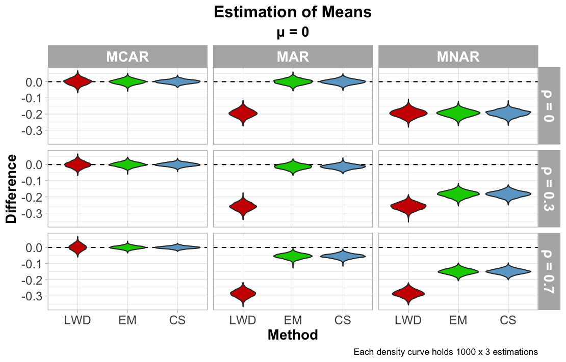
EM and CS perform similarly under MAR, but the bias of its results appear to increase gradually with increasing $\rho$. There are several possibilities as to why this is the case: under the MAR mechanism, the relationship between missing and observed cells are strengthened when collinearity is high. Increased collinearity reduces the effective independent information from other variables, potentially overemphasizing small deviations in the conditional means for CS, and convergence to maximum likelihood loses stability for EM.
MNAR data indicates significant bias for all methods, regardless of the values for $\rho$. Because the MNAR setup keeps the top 90% of each column (independent of the values of other columns), that proportion of the MVN distribution is lost regardless of what the observed values suggest, and without any prior means or belief supplied, the data cannot be reconstructed fully.
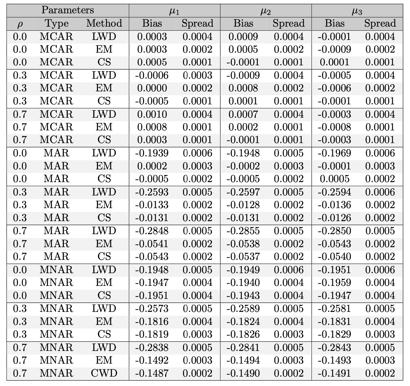
The Table below dives deeper on the mean estimation figure and reports the numerical bias and spread of each method (note how LWD is always higher in spread).
Variance, Covariance, and Correlation Estimation
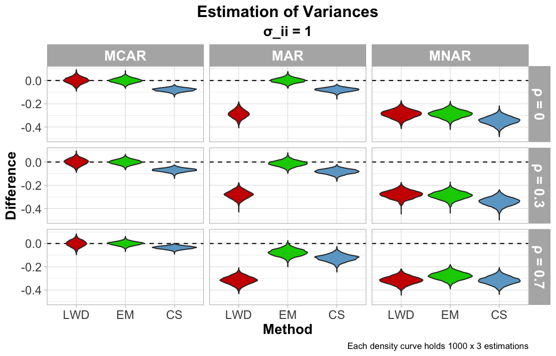
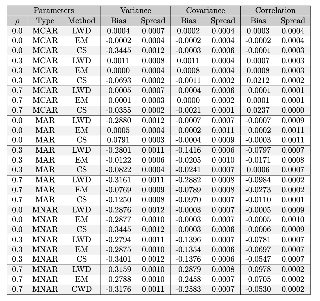
The next figure below reports how each imputation method approximated the variance of each column (or the diagonal values of the covariance matrix). For MCAR, MAR, and MNAR, the CS imputation method approximated the variance with some noticeable bias. This result is likely due to how the missing values are pooled from five different samples. With a pooled approximation for each missing cell, this will likely drive the variance lower than the truth. LWD is also noticably shifted away from approximating the true variance of MAR data, since cutting portions of the data will minimize the range of observed values and reduce variance significantly. Once again, each method returns biased estimations of the variance for MNAR, noticeably less than the true variance.
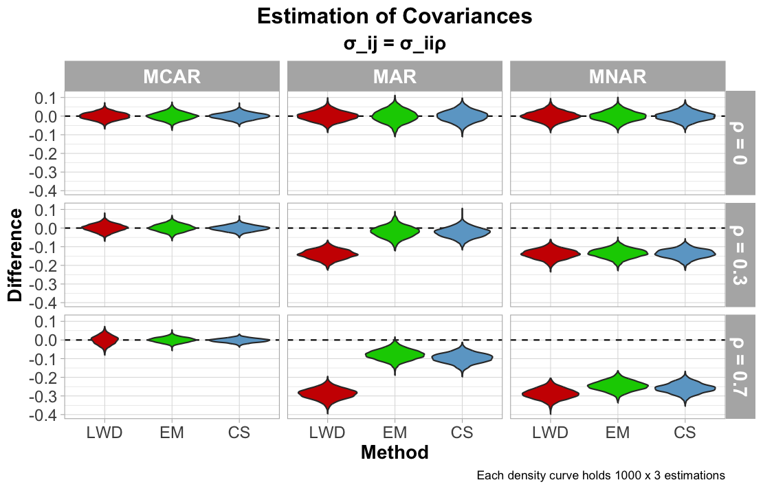
The next figure illustrates performance on estimating covariance. Each method accurately estimated the covariance when the data was MCAR (with less precision from LWD). Increasing $\rho$ for MAR data influences greater biased estimates of the covariance for LWD. For MNAR, the estimations of the covariance greatly increase as $\rho$ increases, suggesting that, even though $\rho = 0$ was accurately estimated, each imputation method cannot truly determine the true covariance.
Calculating correlation involves both the variance and covariance of the columns. Thus, a biased variance or covariance can conclude to an inaccurate estimation of the correlation.
\[\rho_{X_1, X_2} = \frac{\text{Cov}(X_1, X_2)}{\sqrt{\text{Var}(X_1) \cdot \text{Var}(X_2)}}\]The last figure reports approximations of the correlation. As collinearity deviates from 0 for MCAR, CS shifts away from the true correlation, which may be tied to the variance predictions and its inaccuracy in the estimation of the MVN variance. Correlation estimates worsen for LWD (and arguably EM) when the data is MAR and collinearity increases. Imputation methods for MNAR increase its bias in estimating correlation as that correlation increases, which is likely connected to the covariance predictions.
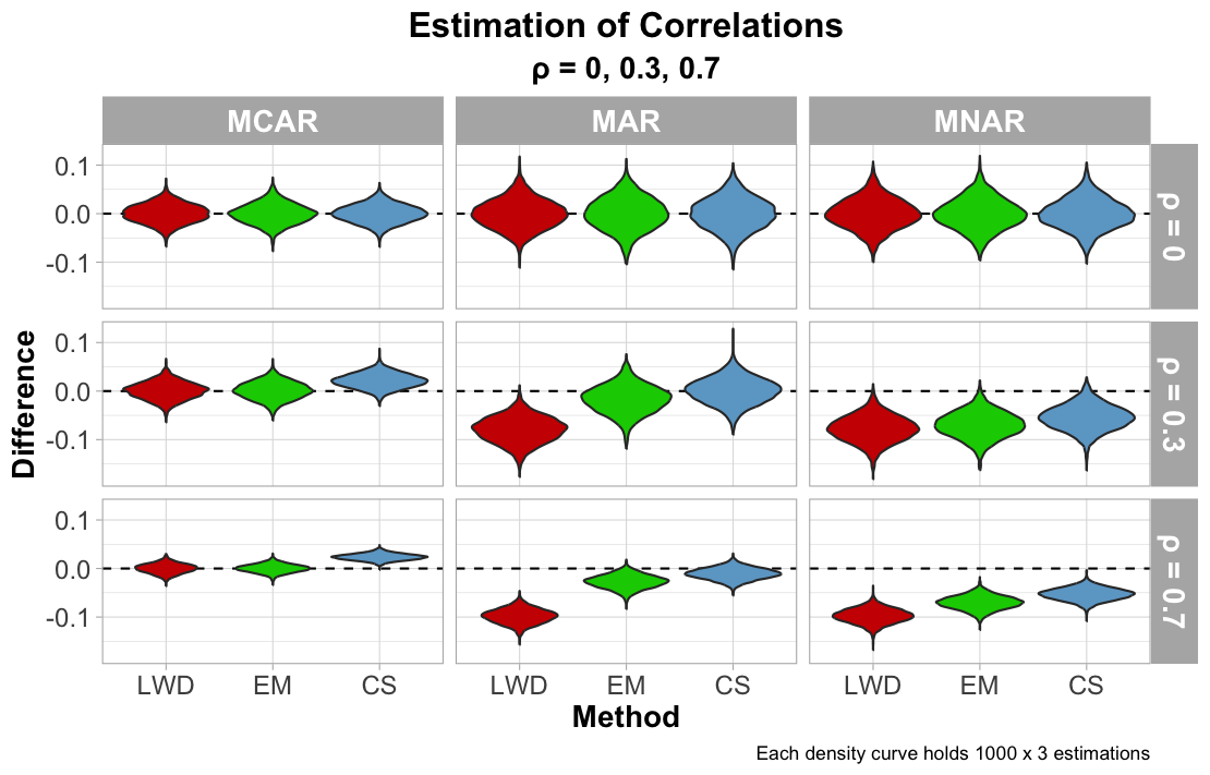
An interesting discovery from evaluating correlation estimates was how the spread of the estimations decrease as $\rho$ increases. The believed explanation for this observation is attributed to how reducing $\rho$ implies little to no linear relationship between variables, which at times these methods may rely on for accuracy. This lack of structure increases the difficulty for imputation methods to accurately estimate the relationship, and consequently estimates of low $\rho$ will show greater spread.
The table below details the variance, covariance and collinearity approximations.
Little’s MCAR Test Results
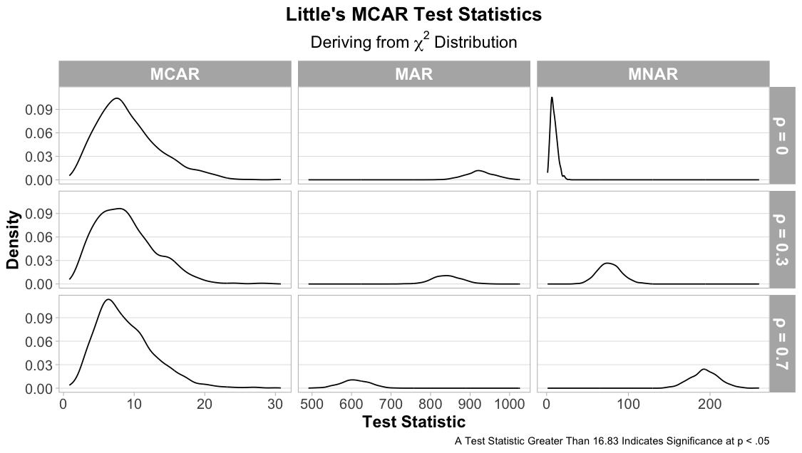
In the final figure below, Little’s MCAR test verifies its ability to distinguish whether missing data is MCAR and MAR. When collinearity is high, however, the test fails to distinguish MNAR from MCAR. This likely happens due to the minimal covariance structure, and the test can only assume that the observed data is not truncated to a proportion of its values. However, the test does improve its ability to differentiate MNAR from MCAR when data is dependent, since the data can now detect a relationship between missing and observed values.
Conclusion
This research evaluated how three unique imputation methods estimate the mean, variance, covariance, and correlation when data is missing and varies in its pattern of missingness. Even though Listwise Deletion (LWD) is computationally efficient and intuitive in programming languages, it estimates variable statistics with considerable bias and uncertainty, particularly when the data is Missing At Random (MAR) and Missing Not at Random (MNAR). Conditional Sampling (CS) outperforms LWD in plenty of the estimations, but increasing collinearity (ρ) trends estimation from CS towards bias.
According to our simulation study, Expectation-Maximization (EM) is the most accurate and reliable method of the three. EM assumes the data to derive from a multivariate normal distribution, and iterates between estimating the expected values of the missing data given current parameter estimates (Expectation-step), and then updating the parameter estimates to maximize the likelihood of the complete data (Maximization-step). This alogrithm performs well for both Missing Completely at Random (MCAR) and MAR data, but fails to approximate data from MNAR data. However, since all methods were flawed at estimating MNAR data, future research may consider other algorithms that can estimate it better.
Little’s MCAR Test proved to be a simplistic yet sound method for identifying whether data was MCAR or MAR. However, when collinearity is low in a dataset, the test struggles to distinguish MCAR from MNAR. The concern for this distinction is inconsequential since variables are rarely completely independent in a given dataset.
Future endeavors may consider additional sensitivity tests to better differentiate whether datasets are MCAR, MAR, or MNAR, as the missingness patterns influence the imputation algorithms and their ability to correct the data. Future simulation studies can also expand upon the idea of collinearity, considering negative $\rho$ values, or in addition generating multivariate normal datasets to have varied dimensions, $\mu$, $\Sigma$, and proportion of missing values $p$. There is additional room for detailing how the imputation methods perform differently when the data does not derive from a multivariate normal distribution, which may prove to be a shortcoming for EM since it assumes the data to be MVN. All in all, imputation methods such as LWD, EM, and CS are considerably prominent tools for the data professional in being able to complete machine learning tasks with accuracy and precision.