Last Updated: 21 Feb 2025
Table of Contents
Introduction
Raw data is almost always messy. It often contains errors ranging from incorrect entries to missing values. Failing to handle these errors can disrupt machine learning algorithms and statistical inference, leading to inflated variance and biased estimates. However, erroneous data often follows certain patterns. In Part 1, we discussed how missing data can be Missing At Random, Missing Completely At Random, or Missing Not At Random — all of which relate to the correlation structure of the data.
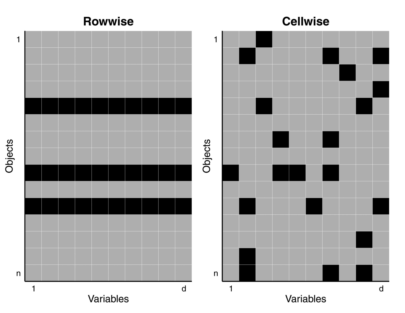
Outliers, on the other hand, fall into two main categories: casewise and cellwise outliers.
Casewise Outliers
Casewise outliers occur when an entire row in a dataframe is anomalous. This assumes that most cases come from a certain model distribution, but some deviate from it. These outliers are relatively easy to detect using methods like Cook’s or Euclidean Distance. A large body of research already exists on detecting these types of outliers.
Cellwise Outliers
Cellwise outliers occur when a single cell within a row is anomalous. These are harder to detect and more common in research data. They often result from data entry errors or recording issues. Research into detecting cellwise outliers is relatively recent, with significant advancements over the last decade by researchers like Rousseeuw and Raymakers. In Part 3, we will explore these methods and introduce a new approach.

Types of Cellwise Outliers
Cellwise outliers are tricky to detect because they only stand out in multi-dimensional settings or when reduced to two dimensions. Without actively looking for them, they can go unnoticed and compromise model performance and statistical inference.
We’ll explore different types of cellwise outliers using a three-dimensional dataset generated from a multivariate normal distribution. The plot below illustrates the dataset’s strong positive correlation between $X_1$, $X_2$, and $X_3$, which makes detecting cellwise outliers easier despite potential issues with linear models.
Type A: Z-Score
A cell value is much larger or smaller than expected. We define $z$ as the number of standard deviations ($\text{SD}(X_i)$) that $X_{ij}$ deviates from the true value.
- Example: A researcher records subjects’ weights, but some are recorded in pounds instead of kilograms.
Type B: Mahalanobis Quantile
A cell value is exchanged with a value within the range of $\sim U[\min(X_i), \max(X_i)]$, causing it to exceed the 99th percentile of the Mahalanobis distance of the uncontaminated data.
- Example: A computer program accidentally shuffles values in one of the columns, disrupting the correlation structure.
Type C: Cellwise Replacement
A cell value is replaced by a specific value. This is based on the function generateData in the cellWise package (Raymaekers and Rousseeuw, 2022).
- Example: A computer program randomly replaces some values in a column with 3 — even though some original values were already 3.
Conclusion
We explored the difference between cellwise and casewise outliers, along with the different types of cellwise outliers and how they appear in real-world data. In Part 3, we will examine how our new algorithm compares to leading methods for detecting cellwise outliers.