Last Updated: 12 Aug 2025
Table of Contents
Introduction
In 2022, NIH researchers published a 2022 study where they put PhDs, statisticians, and other academics to test something they all should know very well: what is hypothesis testing?
Participants were given a short scenario about statistical significance and asked two seemingly simple follow-up questions. These weren’t trick questions, either—just the kind of thing you might hear in any A/B testing meeting.
Here’s the exact setup they saw:
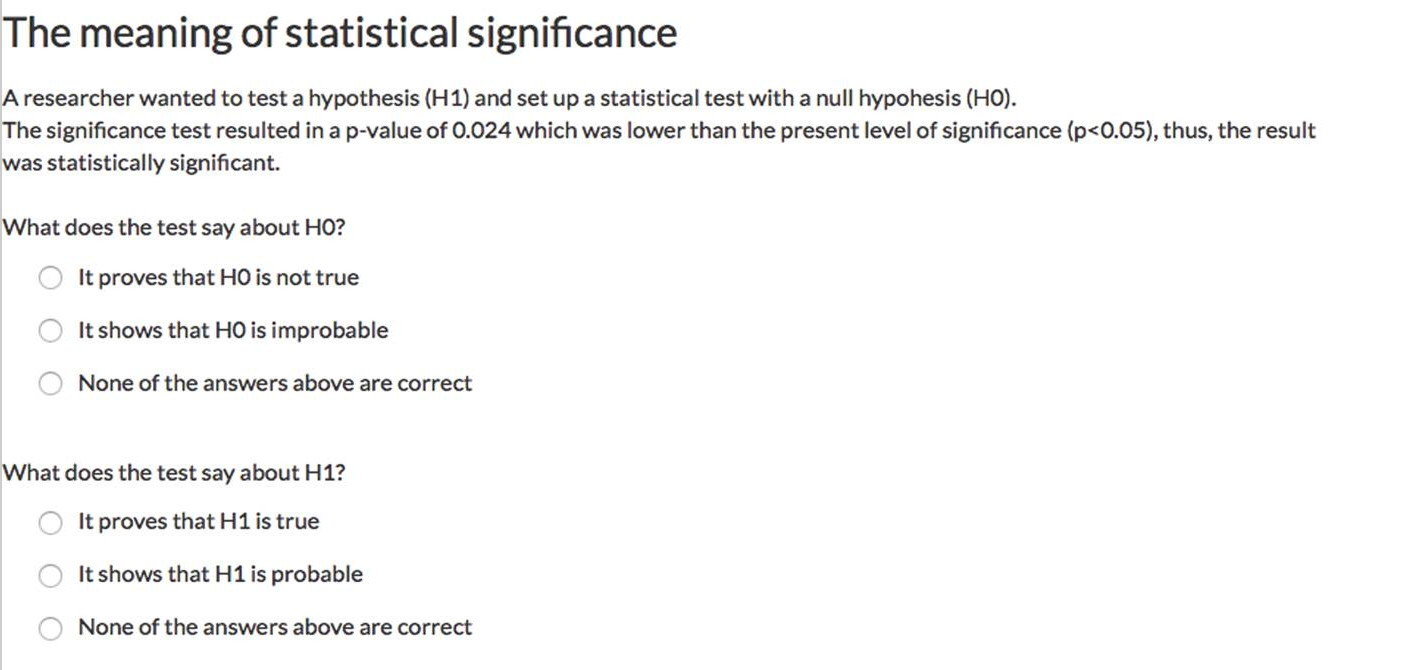
Think you can answer these two questions correctly?
So, why do so many with educations still get this wrong? Because terms like p-value, test statistic, and confidence interval—while central to A/B testing—are widely misunderstood, even among professionals.
A/B testing is built to make comparisons, and our brains naturally want to frame those comparisons in everyday language: Is A better than B? By how much? The classical A/B test—often taught in your first statistics course—answers these questions using only the information in your sample. On paper, it’s straightforward.
But when the statistical jargon enters the room, most people’s mental model breaks down. We confuse “unlikely under H₀” with “probable under H₁,” and we start interpreting confidence intervals as if they were lottery odds.
This post is your crash course refresher. First, we’ll unpack what p-values and confidence intervals actually mean in the frequentist world. Then, we’ll see how Bayesians approach the same problem—an approach that, depending on your style, might feel either more natural or persuasive.
How Frequentists Think
Imagine you’ve run an A/B test on two website designs. You collect data and run a statistical test. Out comes a p-value of 0.03. What’s really going on here?
In the frequentist mindset, the p-value tells you: If there truly were no difference between A and B (the null hypothesis is true), how often would I see a result this extreme—or more extreme—purely by random chance?
To picture it, think of an alternate universe where you could run your experiment an infinite number of times assuming there is no difference. The results of those imaginary experiments form a bell-shaped “sampling distribution.” Your p-value is the proportion of that curve in the “extreme” tail where your observed result lies. If that proportion is tiny, you conclude your data is not consistent with the “no difference” story—and you reject the null hypothesis.
Here’s the catch: rejecting H₀ doesn’t mean you know what’s true instead. You’re essentially saying, This no-difference story doesn’t fit the evidence… but I don’t yet know the full story.
Frequentist methods have a few advantages:
- They’re computationally straightforward and widely applicable.
- Reporting small p-values has become standard in academic publishing.
- Most researchers and analysts at least know what a p-value is supposed to represent.
The biggest stumbling block? Interpretation. People often think a p-value is “the probability H₀ is true” (it’s not), or that a 95% confidence interval means “we are 95% sure the true value lies here” (it doesn’t). The frequentist world is full of subtle rules about what you can and can’t say—and that’s where Bayesians take a very different path.
How Bayesians Think
Let’s switch gears with a simpler example—a coin flip. You flip a coin, catch it, and cover it. You ask both a Bayesian and a frequentist friend:
“What’s the probability that this coin landed on heads?”
- The Frequentist starts with sharing their experience: “I’ve flipped coins like this before—100 flips, and about 50 were heads. So the long-run probability is 0.5.” But when you press them—“Okay, but for this specific coin flip right now?”—they’ll say they can’t give you a probability. From their point of view, the outcome is already fixed as either heads or tails. Probability to them describes long-run frequencies, not single events.
- The Bayesian answers differently. They give their belief, stating “I’ve seen enough fair coins to believe the probability is 50%.” They might also quantify how confident they are in that belief—maybe 95% sure based on thousands of previous flips. Then they’d wait for evidence (actual flips from this specific coin) to update that belief. This is the core of Bayesian thinking: start with prior knowledge, bring in new data, and get a posterior—an updated belief about the probability of heads.
In Bayesian statistics, once you have the posterior distribution, you can answer the kinds of questions people want to ask:
- What’s the probability Group A’s conversion rate is higher than Group B’s?
- What’s the probability the true difference lies between an interval X and Y?
That last one is particularly powerful: a Bayesian 95% credible interval isn’t restricted the same way a Frequentist is: they really do mean that there is a 95% probability the true value lies within—exactly the kind of plain-English interpretation that frequentists have to dance around by stating their “confidence level”.
Of course, there’s a price: Bayesian methods require you to specify a prior belief (which can be controversial), and the math can be computationally heavier. But in exchange, you get results that align much more closely with how humans naturally think about uncertainty.
In the next sections, I will give show the process of how frequentists and Bayesians perform an A/B test in R.
Example: Credit Card Fraud
We’ll use a dataset from Kaggle.
Imagine your boss hands you this data and asks “Is there significant evidence that making more than one purchase on a credit card is a signal for fraud?”
To investigate, we define:
Group A: Multiple-item charges (treatment)
Group B: Single-item charges (control)
Before diving into statistical testing, we start with some exploratory analysis. The bar chart below compares the fraud rates between the two groups:
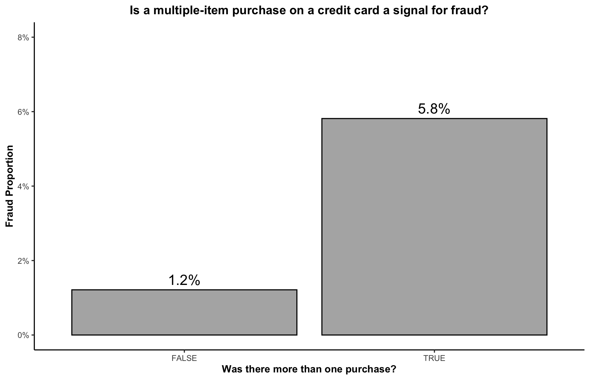
From this plot, multiple-item purchases appear to increase the probability of fraud by 300%. This suggests that the difference is at least eye-catching. We now need to formally test whether this difference is statistically significant.
Frequentist Proportions Testing
Let’s determine whether multiple-item credit card purchases have a significantly higher fraud rate than single-item purchases.
To follow along, download the dataset from Kaggle and run the following setup code:
library(tidyverse) # install.packages(tidyverse)
library(tidymodels) # install.packages(tidymodels)

data <- read_csv("payment_fraud.csv") %>%
  rename(X = numItems, Y = label) %>%
  select(X, Y)

# Convert to binary indicators
data$Y <- ifelse(data$Y == 1, T, F) # fraud?
data$X <- ifelse(data$X > 1, T, F) # >1 purchase?

# Compute group-level stats
group_stats <- data %>%
    group_by(X) %>%
    summarise(Prop = mean(Y), Sum = sum(Y), N = n())
gA <- group_stats[2,] # Multiple-item group
gB <- group_stats[1,] # Single-item group
Step 1. Hypotheses
We begin by stating the null and alternative hypotheses:
- Null $H_0$: $p_A - p_B = 0$ (fraud rates are the same for both groups)
- Alternative $H_1$: $p_A - p_B \neq 0$ (fraud rates differ)
We’ll also choose a significance level, $\alpha = 0.05$, as our decision cutoff.
exp_diff <- 0 # null hypothesis difference
obs_diff <- gA$Prop - gB$Prop
alpha <- 0.05 # cutoff
Step 2: Check Assumptions
The two-proportion z-test assumes:
- Random and independent samples
- Each group has at least 5 (preferably 10) “successes” and “failures”
gA$N * gA$Prop > 5
gA$N * (1-gA$Prop) > 5
gB$N * gB$Prop > 5
gB$N * (1-gB$Prop) > 5
Step 3: Standard Error
- Unpooled: For confidence intervals
- Pooled: For hypothesis testing and p-values
# unpooled (for CI)
SE_u <- sqrt(((gA$Prop) * (1 - gA$Prop)) / gA$N + ((gB$Prop) * (1 - gB$Prop)) / gB$N)

# pooled (for p-value)
p_hat <- (gA$Sum + gB$Sum) / (gA$N + gB$N)
SE_p <- sqrt(p_hat * (1-p_hat) * (1/gA$N + 1/gB$N))
Step 4. Run the test We can calculate the z-score and p-value manually, or use built-in R functions.
Method 1: Manual
z_val <- (obs_difference - exp_difference) / SE_p

# Compute p-value
p_val <- 2*pnorm(q = abs(z_val), lower.tail = F) # multiply by 2 for two-sided
paste("Z-score", round(z_val, 2))
paste("p-value", p_val) # definitely significant

# Compute confidence interval of difference
lwr = obs_difference - qnorm(1-alpha/2) * SE_u
upr = obs_difference + qnorm(1-alpha/2) * SE_u
paste("Observed Difference")
paste(obs_difference)
paste("Observed Difference Confidence Interval:")
paste("[", lwr, ", ", upr, "]", sep = "")
Method 2: base R prop.test()
prop.test(x = c(gA$Sum, gB$Sum), n = c(gA$N, gB$N),
          alternative = "two.sided", correct = F)
Method 3: tidymodels::prop_test()
data %>%
  prop_test(Y ~ X, order = c("TRUE", "FALSE"),
            correct = F, z = TRUE)
Step 5. Conclusion
These methods are consistent in their result: given that the p-value is 8.5e-49 (very very really small) and is less than 0.05, we reject the null hypothesis and conclude that the risk for fraud is significantly higher when multiple-item purchases are made. This p-value also suggests that the probability that there is truly no difference between single-item and multi-item purchases is this low, given the data we had observed.
Bayesian Proportions Test
Here’s where Bayesian thinking really shines. Instead of framing everything around what’s the probability of seeing this data if there’s no difference, we flip the script and ask: What’s the probability that one group really does have a higher fraud rate than the other?
To get there, Bayesians build a probability distribution for each group that reflects both what we believe before seeing the data (the prior) and what the data tells us (the likelihood). Think of it like this:
-
The likelihood comes from the data you’ve collected—how many fraudulent purchases you actually observed. Because each transaction can be fraud or not, the likelihood naturally follows a binomial distribution.
-
The prior captures your belief about the underlying fraud probability before looking at this dataset. Since that probability can only be between 0 and 1, a beta distribution makes a natural choice.
Bayes’ theorem ties these two together into the posterior distribution—your updated belief about the fraud probability after seeing the data:
\[\pi(p | y) \propto f(y | p)\pi(p)\]This posterior is powerful because it tells you directly the range of likely values for $p$, the probability of fraud. Even better: once you have a posterior for Group A and Group B, you can simulate from both and simply count how often $A > B$. In other words, you can compute the actual probability that fraud risk is higher in one group than the other. No careful dance around p-values, just a straight answer to the question decision-makers care about.
The catch? Bayesian A/B testing is computationally heavier than the frequentist plug-and-play tests. Instead of one function call, you usually rely on MCMC simulations (Markov Chain Monte Carlo) to approximate those posteriors. But thanks to modern tools like nimble, Stan, and bayesAB, running these analyses is becoming far easier. Let’s run this in R:
Step 1. Prior Distributions
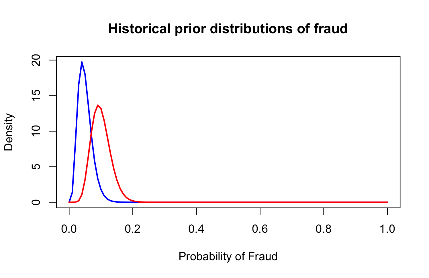
To begin a Bayesian A/B analysis, we first define our prior beliefs. Since fraud is rare but non-zero, I want my priors to reflect this. I also expect that multi-item purchases are more likely to be fraudulent than single-item purchases. With this in mind, I set Beta priors for each group:
-
Group A (multi-item, treatment): $\Beta(\alpha = 10, \beta = 90)$, reflecting a ~10% fraud rate.
-
Group B (single-item, control): $\Beta(\alpha = 5, \beta = 95)$, reflecting a ~5% fraud rate.
If strong priors feel uncomfortable, you can use a “non-informative” prior like $\Beta(1, 1)$, which places equal weight across all possible fraud rates (uniform over 0–1).
# Group = FALSE (~5% are y = TRUE)
f_a_hp <- 05
f_b_hp <- 95

# GROUP = TRUE (~10% are y = TRUE)
t_a_hp <- 10
t_b_hp <- 90

# note hp stands for historical prior, use a=1 and b=1 for "non-informative" prior

# Plot distributions
curve(dbeta(x, f_a_hp, f_b_hp), from = 0, to = 1,
      col = "blue", lwd = 2,
      xlab = "Probability of Fraud",
      ylab = "Density",
      main = "Historical prior distributions of fraud",
      )

curve(dbeta(x, t_a_hp, t_b_hp), from = 0, to = 1,
      col = "red", lwd = 2, add = TRUE)

legend("topright",
       legend = c("X = 1 Purchase",
                  "X = 2+ Purchases"),
       col = c("blue", "red"), lwd = 2, bty = "n")
Step 2. Deriving the Poseterior
Our data are Bernoulli outcomes (fraud vs. no fraud), which means the total number of fraud cases follows a Binomial distribution. Combining the Binomial likelihood with the Beta prior gives a Beta posterior. To prove this:
-
Assume a Beta prior for $p$: \(p \sim \mathrm{Beta}(\alpha,\beta), \qquad \pi(p) = \frac{1}{\mathrm{B}(\alpha,\beta)} \, p^{\,\alpha-1} (1-p)^{\,\beta-1},\)
-
Then, let $y \in {0,1,\dots,n}$ denote the number of successes in $n$ Bernoulli trials with success probability $p$. \(y \mid p \sim \mathrm{Binomial}(n,p), \qquad f(y \mid p) = \binom{n}{y}\, p^{\,y} (1-p)^{\,n-y}.\)
-
The unnormalized posterior (by Bayes’ rule) is \(\pi(p \mid y) \;\propto\; f(y \mid p)\,\pi(p) \;\propto\; \Big[ \binom{n}{y}\, p^{\,y} (1-p)^{\,n-y} \Big] \cdot \Big[ p^{\,\alpha-1} (1-p)^{\,\beta-1} \Big].\) \(\dots \;\propto\; p^{\,(\alpha + y - 1)} \, (1-p)^{\,(\beta + n - y - 1)}.\)
-
We can identify the kernel (Beta) and normalize. \(\pi(p \mid y) = \frac{1}{\mathrm{B}(\alpha + y,\, \beta + n - y)} \, p^{\,\alpha + y - 1} (1-p)^{\,\beta + n - y - 1}.\)
-
Yielding a Beta distribution with new parameters $\alpha^$ and $\beta^$ as \(p \mid y \;\sim\; \mathrm{Beta}\big(\,\alpha + y,\; \beta + n - y\,\big).\)
This is a classic example of a conjugate prior, where the posterior is in the same family as the prior. The beauty of conjugacy is that updating beliefs is as simple as plugging in the observed counts. For fraud risk, that means our updated posterior for each group is just a Beta distribution with parameters adjusted by the data.
Step 3. Testing Treatment Differences
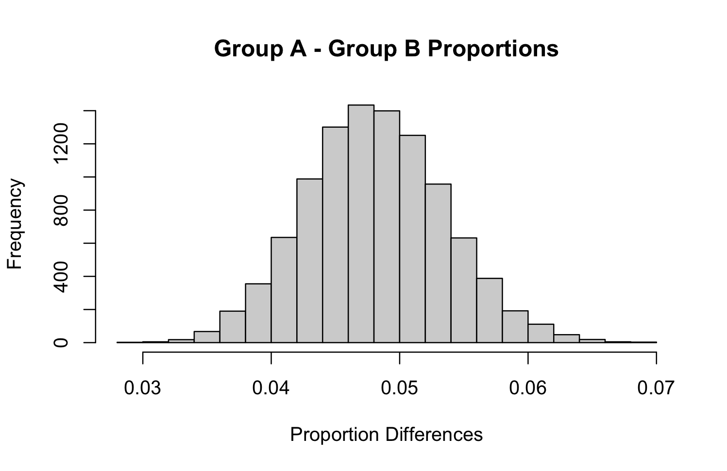
Having separate distributions for each group is helpful, but we need a distribution that models the difference in fraud rates. Unfortunately, no closed form exists for a difference in proportions. To create this, we use simulation.
This can be done directly via random sampling (Method 1), or with MCMC approaches like Metropolis–Hastings (Method 2), which are useful when posteriors don’t have closed-form solutions. For convenience, you can also use packages like bayesAB (Method 3), which handle the computation and visualization.
Method 1: Direct Sampling
# create Group A poseterior parameters
t_s <-  sum(data$Y[data$X == T])
t_astar_hp <- t_a_hp + t_s # historical
t_n <- length(data$Y[data$X == T])
t_bstar_hp <- t_b_hp + t_n - t_s #historical

# create Group B posterior parameters
f_s <- sum(data$Y[data$X == F])
f_astar_hp <- f_a_hp + f_s # historical
f_n <- length(data$Y[data$X == F])
f_bstar_hp <- f_b_hp + f_n - f_s

# distribution of differences
gA <- rbeta(10000, t_astar_hp, t_bstar_hp)
gB <- rbeta(10000, f_astar_hp, f_bstar_hp)
hist(gA - gB, main = "Group A - Group B Proportions",
     xlab = "Proportion Differences")
Method 2: Metropolis Hastings - Gibbs Sampling
For more on this process, I recommend this article. But using Metropolis Hastings or Gibbs sampling is useful in the Bayesian setting when one, the posterior distribution is not a closed form solution, and two, you want good exploration of the parameter space. I won’t explore it further here, but the code snippet below reveals how a Metropolis Hastings framework functions in the proportions test:
n_iters <- 1000
x <- c(t_s, f_s)             # successes
a_prior <- c(t_a_hp, f_a_hp) # Beta prior alpha
b_prior <- c(t_b_hp, f_b_hp) # Beta prior beta
n <- c(t_n, f_n)             # total trials
J <- length(x)

theta_samples <- matrix(NA, nrow = n_iters, ncol = J)
theta_current <- rep(0.5, J)   # initialize at 0.5 for each group

# MH proposal standard deviation (tune this!)
proposal_sd <- 0.2

# function to compute log-posterior density
log_posterior <- function(theta, x, n, a, b) {
  if (theta <= 0 || theta >= 1) return(-Inf) # invalid
  log_lik <- dbinom(x, size = n, prob = theta, log = TRUE)
  log_prior <- dbeta(theta, a, b, log = TRUE)
  return(log_lik + log_prior)
}

for (i in 1:n_iters) {
  for (j in 1:J) {

    # propose new theta via logit-normal random walk
    logit_theta <- qlogis(theta_current[j])                  # current on logit scale
    logit_theta_prop <- rnorm(1, mean = logit_theta, sd = proposal_sd)
    theta_prop <- plogis(logit_theta_prop)                   # back-transform

    # log-posterior for current and proposed
    log_post_current <- log_posterior(theta_current[j], x[j], n[j], a_prior[j], b_prior[j])
    log_post_prop <- log_posterior(theta_prop, x[j], n[j], a_prior[j], b_prior[j])

    # symmetric proposal, so acceptance ratio simplifies
    log_accept_ratio <- log_post_prop - log_post_current

    if (log(runif(1)) < log_accept_ratio) {
      theta_current[j] <- theta_prop  # accept
    }

    theta_samples[i, j] <- theta_current[j]
  }
}
Method 3: Use bayesTest() from bayesAB
library(bayesAB)
t_data <- as.numeric(data$Y[data$X == T])
f_data <- as.numeric(data$Y[data$X == F])

abtest <- bayesTest(t_data, f_data,
          priors = c('alpha' = f_a_hp, 'beta' = f_b_hp),
          distribution = 'bernoulli')

summary(abtest)
Step 4. Conclusion
To get your “Bayesian p-value”, you do the following (assuming you used method 1):
my_test <- mean(gA > gB)
print(paste("Probability that group A > group B in TRUE cases:", my_test))
ci <- quantile(gA - gB, probs = c(.025, .975))
paste("[", ci[1], ", ", ci[2], "]", sep = "")
To summarize the results, we calculate:
-
$P(p_A > p_B)$, the probability that multi-item purchases have higher fraud risk.
-
A 95% credible interval for the difference $p_A - p_B$.
In our case, the probability that Group A exceeds Group B is essentially 100%, with the credible interval for the difference around 3.8% to 5.9%. This aligns closely with frequentist confidence intervals, but the interpretation is far more intuitive.
Instead of saying “if we repeated this experiment infinitely, 95% of the intervals would contain the true difference”, we can directly say “given our data and prior, there is a 95% probability that the true difference lies within this interval.”
That’s the real advantage of the Bayesian framework: it allows us to make probabilistic statements about the parameters we care about, in the exact way we want to think about them.
Conclusion
At the heart of this article was the challenge of interpreting significance tests—something that often feels abstract or even misleading when framed in the frequentist hypothesis testing paradigm. By contrasting this with the Bayesian approach, which lets us talk directly about the probability of one group being riskier than another, we saw how interpretation can become much more intuitive. Using a fraud detection dataset, we walked through how both frameworks address the same question—whether multi-item purchases carry higher fraud risk—and found consistent answers, despite the different philosophies. The key takeaway is that neither framework is inherently “better”; Bayesian methods may offer more natural interpretations while frequentist methods remain computationally simpler and widely used. Ultimately, whichever approach you choose, both can provide valid, actionable insights if applied carefully.