Last Updated: 25 May 2026
Table of Contents
Abstract
How much taller do women prefer their romantic partners to be — and what factors influence that preference? Using survey data collected from college-aged women in Utah County, this project investigates the relationship between behavioral, demographic, and lifestyle variables and preferred male height differences. Rather than treating responses as exact values, I modeled height preferences using a Bayesian latent Gaussian framework that accounts for the fact that survey responses are discretized approximations of underlying continuous preferences. Results suggest that women who are shorter, go on more dates, work out more frequently, visit soda shops more often, and lean more politically conservative tend to prefer larger height differences in partners.
Introduction
Modern dating culture is shaped by a complex combination of physical attraction, lifestyle compatibility, social expectations, and online interactions. Among these preferences, male height consistently emerges as one of the most discussed characteristics in heterosexual dating preferences. Prior research has shown that taller men are often perceived as more attractive, and many women report preferring partners taller than themselves.
But while height preferences are commonly discussed, an interesting statistical question remains:
What factors are associated with stronger or weaker preferences for taller partners?
To investigate this, I analyzed survey responses collected through the Latter-day Stats Instagram page from college-aged women living primarily in Utah County. The project combines Bayesian statistics, latent variable modeling, and probabilistic prediction to study how individual characteristics relate to preferred partner height differences.
Data Description
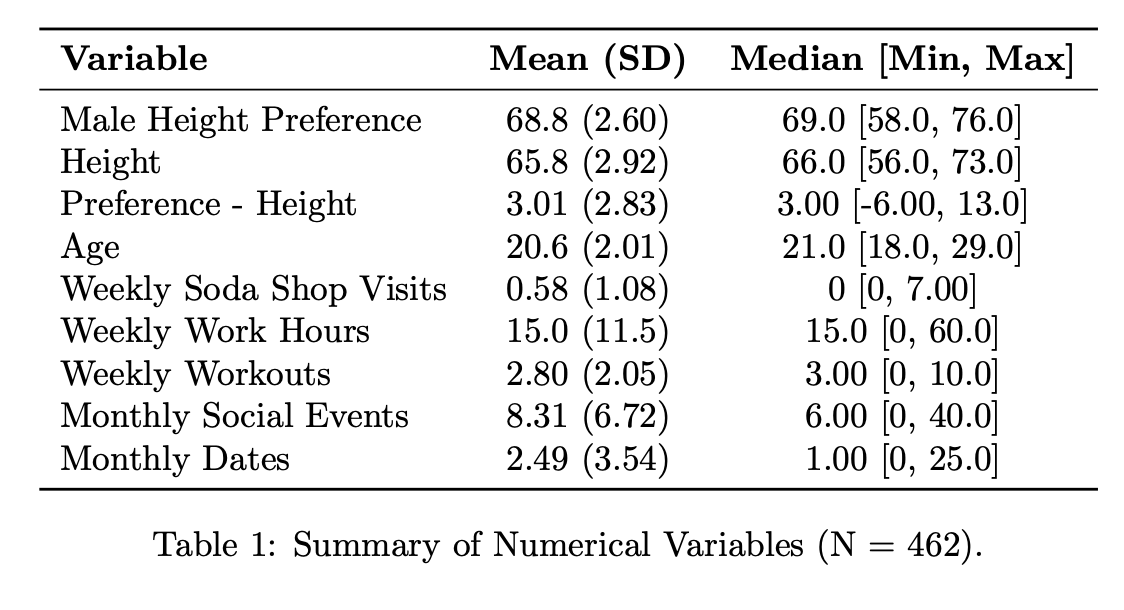
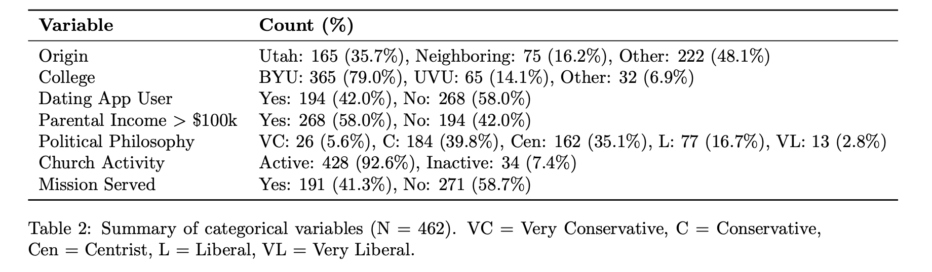
The original survey contained over 1,000 respondents and included dozens of questions covering dating behavior, religion, politics, lifestyle habits, education, and demographics. After cleaning the data and restricting the sample to the target population, the final analysis included 462 college-aged women.
The primary response variable was the preferred male height difference, or in other words, the minimum acceptable male height relative to the respondent’s own height (measured in inches).
The average preferred difference was approximately 3 inches taller than the respondent.
Key predictors included:
- Respondent height
- Political philosophy
- Dating app usage
- Weekly workouts
- Monthly dating frequency
- Weekly soda shop visits
- Religious activity
- Geographic origin
- Work hours and social activity
Several count-based variables were log-transformed and standardized prior to modeling to improve interpretability and statistical stability.
Methodology
One challenge with modeling height preferences is that survey responses are recorded as integers, even though actual preferences are likely continuous. For example, if someone reports preferring a partner “3 inches taller,” their true preference may realistically be anywhere near that value rather than exactly 3.000 inches.
To account for this, I used a Bayesian latent Gaussian model.
Let $Y_i$ denote the observed integer-valued response for respondent $i$, representing the minimum acceptable male height difference relative to the respondent’s own height.
Instead of assuming $Y_i$ is the true preference itself, we assume it is generated from an unobserved continuous latent variable $Z_i \sim N(\mu_i, \sigma^2)$, where $\mu_i = X_i^\top \beta$.
Thus the observed response $Y_i$ arises through discretization:
\[Y_i = y_i \iff Z_i \in [y_i - 0.5,\; y_i + 0.5)\]This means that if someone reports preferring a partner “3 inches taller,” the model interprets this as their true latent preference lying somewhere in the interval $[2.5, 3.5)$ rather than exactly 3.000 inches.
Under this framework, the likelihood contribution for observation $i$ becomes:
\[P(Y_i = y_i \mid X_i) = \Phi\left( \frac{y_i + 0.5 - \mu_i}{\sigma} \right) - \Phi\left( \frac{y_i - 0.5 - \mu_i}{\sigma} \right)\]where $\Phi(\cdot)$ is the cumulative distribution function of the standard normal distribution.
Rather than predicting an exact outcome, the model estimates the probability mass assigned to each integer-valued interval. Interestingly, in terms of predictability, the Bayesian Latent Gaussian model has almost exactly the same accuracy as normal linear regression. This implies that discretization does not substantially distort the conditional mean structure of the response. However, the latent Gaussian model remains preferable because it provides a statistically coherent framework for modeling discrete survey responses generated from underlying continuous preferences.
Results
Interpreting Coefficients
This figure below shows the simulated curves of each variable and their influence on the preferred height gap. In this case, any distribution highlighted red has a significant negative impact, while those highlighted blue are positively influential.
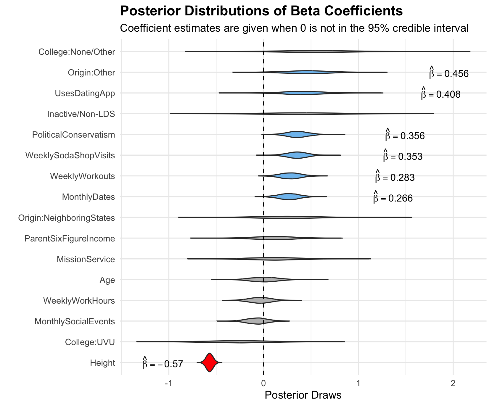
The strongest predictor by far was the respondent’s own height. Taller women tended to prefer partners closer to their own height, while shorter women preferred larger height differences: numerically, every one-inch increase in a girl’s height lead to over half-inch decrease in this gap Respondent height alone explained roughly 82% of the explainable variation in relative height-gap preferences.
The other 18% derives from the following behavioral features, which also showed meaningful associations with height preferences:
- Every one-level increase in political conservatism leads to an expected 0.34 inch increase [95% CI: 0.14, 0.57]. Very Liberal to Very Conservative $\approx$ 2 inch increase.
- Using a dating app leads to expected 0.42 inch increase [0.00, 0.84].
- Individuals from outside of Utah and neighboring states compared to Utah has an expected 0.46 inch increase [0.01, 0.90].
- Increasing from zero to one date per month has a 0.24 [.05, 0.44] inch increase. This effect has diminishing returns, since going from nine to ten dates per month raises the gap to 0.03 [0.01, 0.06] inches.
- Increase from zero to one workouts per week → 0.29 [0.08, 0.51] inch increase. Zero to five workouts per week leads to 0.75 [0.20, 1.35] inch increase (diminishing returns).
- Having zero to one dirty soda per week leads to 0.50 [0.20, 0.78] inch increase. Zero to three dirty sodas per week → 1.00 inches [0.41, 1.56] inch increase (diminishing returns).
Ultimately, these factors have a significant impact on a girl’s preferred male height gaps, but note that all of these variables are not nearly as influential as her own height.
Interpreting Predictions
This next figure a guess on the preferred male height for two of our subjects. Essentially, the left figure represents the unobservable normal curve for each person, and where on the probability scale a given height preference may exist. The right figures are discretized/rounded to the nearest inch.
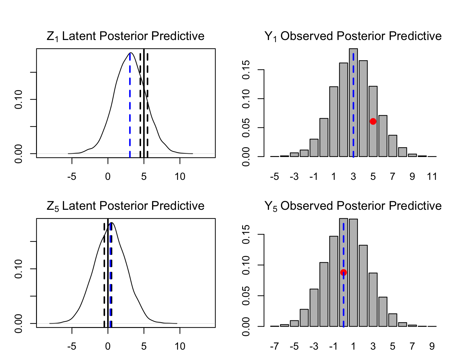
These examples are based on out-of-sample predictions. We highlight two individuals to illustrate different scenarios.
-
For subject 1, a married individual of height 5’7”, the red point represents the observed height difference with their partner ($Y_1 = 5$ inches). Under the model, the probability that the latent preference falls within the corresponding interval is $P(Z_i \in [4.5, 5.5))=$ 12.43%. Overall, the probability that her partner would satisfy the preference threshold (i.e., $Z_i < 5.5$) is approximately 86.61%. This suggests that the observed partner height is consistent with a relatively high-probability region of the individual’s inferred preference distribution.
-
For subject 5, a 5’9” individual, the red point represents their stated preferred height difference. The posterior mean $\mu_i \approx 0$ (blue dashed line) aligns closely with the observed value, indicating that the model assigns relatively high probability mass to this outcome, which is $P(Z_i \in [-0.5, 0.5))=$ 17.15%. Just like for subject one, the model allows us to evaluate the probability that a given partner height satisfies the individual’s preference. For this case, a partner of equal height corresponds to approximately a 53.33\% probability of meeting the preference threshold, while a partner who is 3 inches taller will meet the threshold with a probability of approximately 92.45%.
These predictive summaries highlight how the model can be used to translate estimated latent preferences into interpretable probabilities of observable values.
Conclusion
This project demonstrates how Bayesian latent variable models can provide both predictive accuracy and richer interpretability when analyzing discretized survey responses. While standard regression performed similarly in raw prediction accuracy, the latent Gaussian framework more naturally captures the uncertainty and interval-based nature of reported preferences.
Substantively, the analysis found that preferred partner height differences vary systematically across individuals. Respondent height explained most of the variation, but behavioral and cultural factors — including dating frequency, workout habits, political ideology, and soda shop visits — also showed meaningful associations.
Of course, these findings are observational rather than causal, and the sample reflects a highly specific population centered around Utah County culture. Still, the project highlights how modern statistical modeling can uncover subtle patterns in human preferences while providing interpretable probabilistic insights into dating behavior.